ZHAO Jinping, CAO Yong, SHI Yanyue, and WANG Xin

Mathematical Proof of the Synthetic Running Correlation Coefficient and Its Ability to Reflect Temporal Variations in Correlation

ZHAO Jinping1), 2), *, CAO Yong1), SHI Yanyue3), and WANG Xin1)

1),,266100,2),,266100,3),,266100,

The running correlation coefficient (RCC) is useful for capturing temporal variations in correlations between two time series. The local running correlation coefficient (LRCC) is a widely used algorithm that directly applies the Pearson correlation to a time window. A new algorithm called synthetic running correlation coefficient (SRCC) was proposed in 2018 and proven to be reasonable and usable; however, this algorithm lacks a theoretical demonstration. In this paper, SRCC is proven theoretically. RCC is only meaningful when its values at different times can be compared. First, the global means are proven to be the unique standard quantities for comparison. SRCC is the only RCC that satisfies the comparability criterion. The relationship between LRCC and SRCC is derived using statistical methods, and SRCC is obtained by adding a constraint condition to the LRCC algorithm. Dividing the temporal fluctuations into high- and low-frequency signals reveals that LRCC only reflects the correlation of high-frequency signals; by contrast, SRCC reflects the correlations of high- and low-frequency signals simultaneously. Therefore, SRCC is the appropriate method for calculating RCCs.

running correlation coefficient; synthetic running correlation coefficient; time window; comparability; standard value

1 Introduction

Correlation describes the degree of consistency between two time series. The correlation coefficient (CC) is an im- portant statistical quantity (Pearson, 1896) that reflects the overall correlation between two data series. Because know- ledge of temporal variations in correlation may sometimes be useful, the running correlation coefficient (RCC) was proposed to reflect varying correlations (Kuznets, 1928).

In most cases, RCC simply applies the CC to a pair of data pieces of the complete dataset. The length of the data piece is called the time window, and the window is moved stepwise to obtain the RCC (., Kodera, 1993). RCC is a time series with values greater than −1.0 and less than +1.0. The RCC obtained by this method was called local running correlation coefficient (LRCC) by Zhao. (2018). LRCC is widely used to study varying correlations between two time series, such as the correlations of the Arctic Oscillation and sea level pressure (Zhao., 2006), water transport in the Labrador Sea and the North Atlantic Oscillation (Varotsou., 2015), atmospheric circulation and air temperature (Hynčica and Huth, 2020), Australian rainfall and El Nino (Brown., 2016), solar variability and paleoclimate records (Turner., 2016), equatorial quasi-biennial oscillations and stratospheric tem- peratures (Kodera, 1993; Soukhearev, 1997), solar cycle (Salby., 1997), and solar UV irradiance (Elias and Zossi de Artigas, 2003).

Zhao. (2018) observed that the LRCC algorithm uses the mean values determined by the data within the time window, which means the mean values also vary withtime. LRCC only reflects the correlation of anomalies corresponding to the means and does not reflect the correlation between varying means. Therefore, the authors proposed a new algorithm for RCC called synthetic running correlation coefficient (SRCC). SRCC reflects correlations for anomalies and means using the global means calculated for the whole dataset. The relationship between LRCC and SRCC could be derived to illustrate the consistency and differences of these two algorithms. Some au- thors, such as Zhao. (2019) and Ji and Zhao (2019), have obtained remarkable results using SRCC.

The definition, calculation method, application examples, and physical significance of SRCC were addressed by Zhao. (2018) in effort to prove that the method is valid and credible. However, SRCC still lacks the support of mathematical theory. In the present study, the validity of SRCC is demonstrated theoretically. The analysis basedon geometric and physical significances proves that SRCC is an appropriate method for measuring varying correlations. In Section 2, the background of the two RCCs is introduced. Comparability as the basic requirement for RCCs is then proposed in Section 3. A mathematical de- monstration of SRCC is given in Section 4. Finally, the physical significance of SRCC is discussed in Section 5.

2 Background of Running Correlation Algorithms

All of the CCs discussed in this study are linear correlations; nonlinear correlations (., Geng., 2018) are not discussed. A simple CC defined as the Pearson pro- duct-moment correlation coefficient (Pearson, 1896) was first introduced by Francis Galton (, 1888) forlinear correlation. The more common form of this CC was developed and applied by Karl Pearson (. For two time series of data leng- thswith equal intervals:

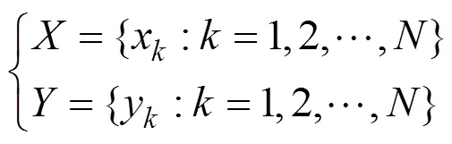
The simple correlation coefficientis written as follows:

where

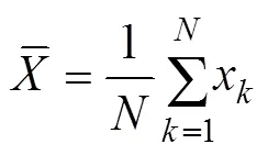
are the means calculated based on all data; thus, these means are called ‘global means’.in Eq. (2) calculated from all of the data is referred to as the ‘global CC’.

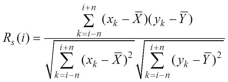
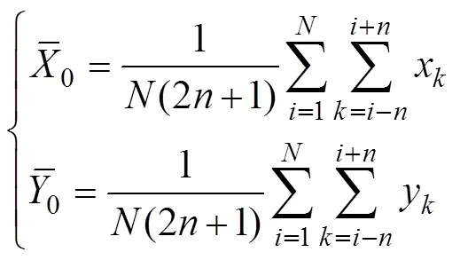
RCC is a useful tool for understanding temporal variations in the correlation between two time series. The CC of two time series centered atis:

whereÎ[1+,−] and the time window is [−,+]; that is:

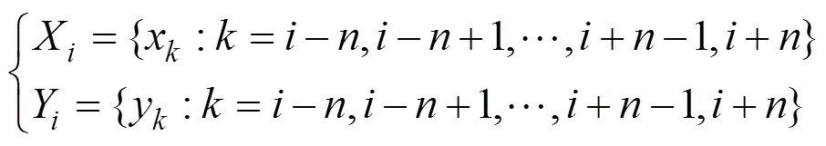
An RCC is obtained by moving the window.R() is LRCC to distinguish it from other RCCs. The means of LRCC are obtained from the data within the time window:

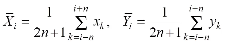
Hereafter, these means are referred to as ‘local means’.

The algorithm for LRCC in Eq. (4) is the direct application of the definition of the global CC. This algorithm only changes the data length with the limit of the time window. The algorithm assumes that the definition used for the global CC could also be applied to the RCC, but no theoretical evidence proving that this direct application is reasonable has been obtained. Zhao. (2018) indicated that the means in Eq. (6) also vary with time. LRCC reflects only the correlation between two anomalies with- in the time window and does not capture the contributions of two varying means. Some important signals contained in the means are clearly missing, which raises further issues whether LRCC reflects the significance of statistics despite ignoring variations in the local means. The RCCs in different time windows should be comparable to each other; however,R() is obtained only from the data with- in the time window and independent of the data of other time windows. Thus, LRCCs in different windows lack common information and, therefore, are not comparable.

Zhao. (2018) identified this problem and proposed a new algorithm to calculate RCC:

Although SRCC was first proposed by Zhao. (2018), this algorithm has actually existed for a long time in the following form:

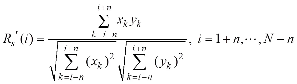
where the means of the two data serieshave been removedbeforehand and the calculation in Eq. (9) does not include the means. This procedure is equivalent to adopting the global means. Therefore, the algorithm in Eq. (9) is equi- valent to SRCC.

Zhao. (2018) attempted to prove which RCC is better by proposing and adopting a criterion, that is, the tem- poral average of the RCC should be close to the global CC. In fact, the average RCC is not exactly equal to the global CC because the amounts of data used for both algorithms differ but could be very close to each other. In general, the temporal average of SRCC is close to the global CC; by contrast, in most cases, the temporal average of LRCC cannot fulfill this criterion.Thus, according to the temporal average criterion, SRCC is better than LRCC for measuring running correlations.

3 Comparability of the RCC Values of Different Windows

An RCC is meaningful only when its values at different times are comparable with each other. For example, if the temperatures of two cities are compared, a large RCC should reflect a consistent variation, and a low one should reflect lower consistency. In this situation, the RCCs are comparable. The standard for each city, which should be an unchanged constant, must be established in advance to meet the requirement of comparability. In the above example, the mean air temperature of each city is used as the comparison standard for cold or warm events, and these events should differ between southern and northern cities. If the standard changes over time, for example, if different temperatures for summer and winter are selected as standards, the RCCs in winter and summer would not be comparable.

Mathematically, a physical component can be decomposed into standard and comparative quantities. The standard quantities should be two unchanged constants not in- volved in the comparison, and the comparison is conducted on the two comparative quantities (Burdun and Markov, 1972). The means of the temperatures are qualified standard quantities for indicating whether the environment is warmer or cooler at a given time. The comparison is applied to the anomalies of the temperature obtained by subtracting the standard quantities. Here we derive the standard quantities mathematically.

That the means ofFand Fare equal to zero is proposed here as a new constraint:

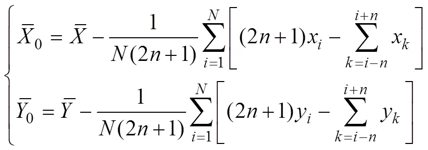
Notice that the range ofis [1, N] and that ofis [1+,−] in Eq. (10). The range ofmust be extended to [1,]. Therefore, the time series={x:=1, 2, …,} and={y:=1, 2, …,} must be extended beyond both limits:

Although any extension could be applied because the extended data do not affect the SRCC calculation in Eq. (7), the extension must satisfy the condition that the mean of the extended data equals the mean of the original data series. This condition is necessary to adopt the same signal of the original data in the extended data. The ideal method is to perform a periodic extension, which is equi- valent to a circular extension (., Woods and Oneil, 1986). The general periodic extension is a sinusoidal extension (., Huybrechs, 2010); it may also be a cosinoidal extension, such as the mirror extension of Zhao and Huang (2001).

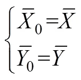
Because the means are unchanged after data extension, the sums of the second terms on the right-hand side of Eq. (13) are always zero. Thus, the unique standard, which is different from the arbitrary standard, is:

For further comparison, an example with two randomly generated white noise data series,1() and2(), for the time range 0–500 is shown in Figs.1a and 1b. The global CC between the two white noise data series is zero, and the average values of LRCC and SRCC are 0.01 and 0.02, respectively. LRCC and SRCC for these two white noise data are quite similar, as shown in Figs.1c and 1d, respectively.

If a constant value is added between 150 and 350, the two time series are defined as:

The constants1and2are set as:

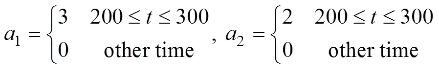
Fig.1 Two running correlation coefficients of a white noise data series. (a) and (b), Two series of white noise (red lines) and the local means (blue lines); (c), LRCC; (d), SRCC.

The new time series are shown in Figs.2a and 2b. The global correlation coefficient is 0.548. RCCs in the time interval with non-zero constants may be expected to show high correlations. SRCC remarkably increases in the pre- sence of these constants and shows an average value of 0.518. By comparison, LRCC changes minimally, as shown in Fig.2c, with an average value of only 0.030. Therefore, whereas SRCC is a suitable metric that could reflect the expected running correlation, LRCC appears to lose important information.

Fig.2 Two running correlation coefficients. (a) and (b), Two series defined by Eq. (15) (red lines) and the local means (blue lines); (c), LRCC; (d), SRCC.

Therefore, from the perspective of comparability, an in- variant value must be chosen as the standard value. Because the local mean varies with time, LRCC is not a comparable CC. The global mean is a qualified and uni- que standard value, and SRCC is the unique RCC satisfy- ing the comparability criterion.

4 Mathematical Difference Between LRCC and SRCC

Although SRCC has been proven to be a qualified RCC by Zhao. (2018) and a unique form of an RCC with comparability as demonstrated in Section 3, mathematically verifying that SRCC is a unique form of RCC based on the original geometric definition of statistical quantities remains necessary.

In the linear correlation framework, a linear correlation can be used to calculate the CC. Consider a pair of time series in Eq. (1) with data lengthin a scatterplot in–y space and draw a straight line through this cloud of points that approaches all of the points ‘as closely as possible’.

If+is used to estimateand+is used to estimate, then the deviations of the two lines from the data are:

Calculating the minimum value of(,) by the least- squares method yields:

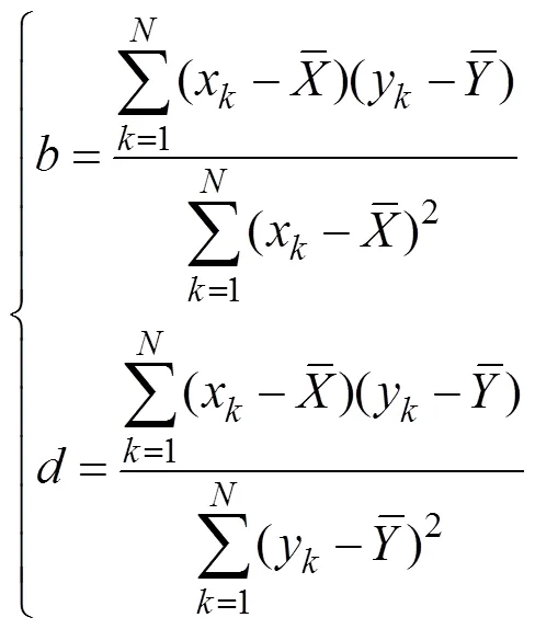
The global correlation coefficientcan be expressed as:

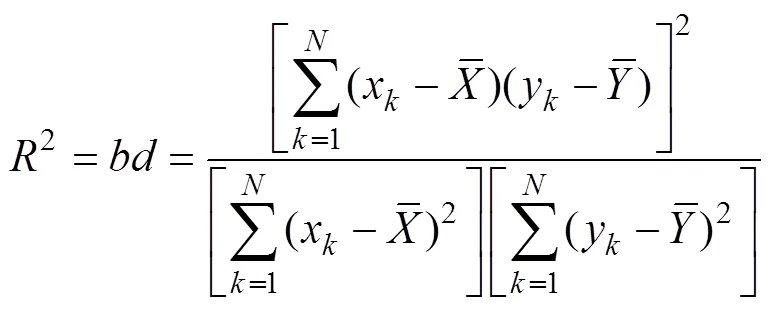
which is identical in form to Eq. (2). Fig.3 shows that the two empirical regression lines pass through the global means ().

LRCC expresses the correlation of the data series in the time window [−,+] as shown in Eq. (5). The linear regression of the data is calculated using a similar method. Here,+is used to estimate,+is used to estimate, and the deviations of the two lines from the data are:

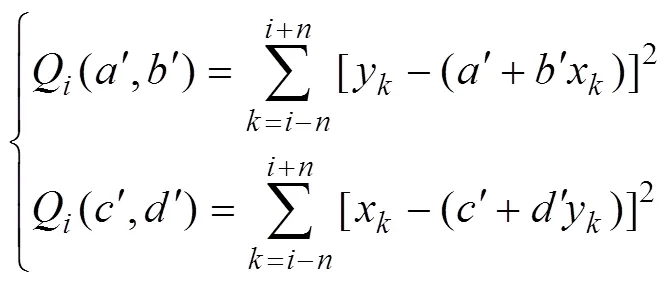
where quantities marked ‘’ are constants related to the length of the time window. The least-squares method can be used to calculateandas follows:

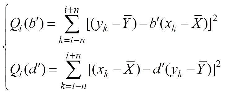
Fig.4 Geometric interpretation of two RCCs at different times t1 and t2. (a), LRCC with different means and ; (b), SRCC with the same means. The shadow area represents the scatterplot of the data.

When the minimumQ()and Q() are calculated by the least-squares method:

Thus:

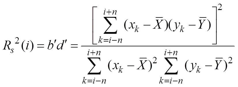
which is the expression for SRCC.

5 Physical Significance of the SRCC

The comparability and geometric consistency of SRCC were demonstrated in Sections 3 and 4 to improve the un- derstanding of the physical significance of SRCC. The following examples present the differences between LRCC and SRCC and explain the reasons behind these differences. Because the annual variation is generally the strongest signal in geoscience, all of the data series used in the following examples are averaged by a 12-point running mean to filter the annual signal.

1) Contribution of the means and the anomalies of SRCC

The relationship between SRCCR()and LRCC R() was simply expressed by Zhao. (2018) as follows:

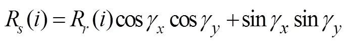
where:

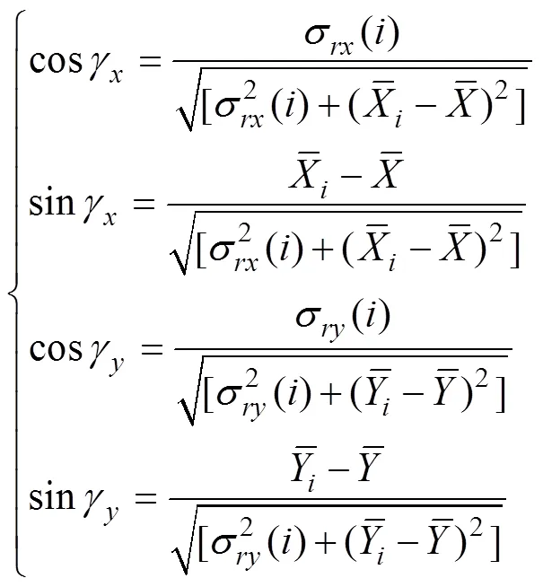
Eq. (27) reveals that SRCC comprisesR() and 1 with certain weights. The weight ofR() is cosγcosγ(cosine- weight), and the weight of 1 is sinγsinγ(sine-weight). A larger variance benefits the cosine-weight, and a larger mean difference benefits the sine-weight. When the mean difference is zero in extreme cases, the two correlation co- efficients are equal; by contrast, when the variance of the anomaly approaches zero, SRCC equals 1.

As an example, the averaged air temperature anomalies for the North Atlantic at 2m and 500hPa and their means are shown in Figs.5a and 5b. LRCC presents a high-fre- quency variation (Fig.5c), whereas SRCC shows a positively dominant running correlation (Fig.5d). Figs.5e and 5f reveal that sine-right is dominant in most time windows and that cosine-right is only apparent in some years. When cosine-right is apparent, SRCC becomes weak or opposite; otherwise, it is strong and close to 1. When the variance is dominant, the anomalous variation is dominant,and the variation of the mean is neglected. When the mean difference is dominant, the variations in anomalies are not important. This example shows that SRCC reflects the com- bined effects of the variance and mean difference simultaneously.

2) Contribution of low- and high-frequency signals

Besides the contributions of the means and anomalies, the double-frequency signal is another factor that decisivelyimpacts LRCC and SRCC. Although fluctuations may contain various frequencies, all of the frequencies considered in the present example can be roughly divided into two groups: one with a period shorter than the time window (high frequency) and the other with a period longer than the time window (low frequency). LRCC usually represents the correlation between high-frequency signals because the low-frequency signals included in the local means are removed from the calculations. By contrast, SRCC still considers the correlation of low-frequency signals. For example, the Arctic Oscillation Index (Fig.6a) and the la- tent heat flux in the Greenland Sea (Fig.6b) are compared The appearances of LRCC (Fig.6c) and SRCC (Fig.6d) are quite similar, which means high-frequency signals do- minate the data set. This result indicates that the latent heat responds better to the high-frequency variations ra- ther than the low-frequency variations of the Arctic Oscillation. According to Eq. (27), cosine-right is dominant in this example. However, the LRCC and SRCC results of 2m and 500hPa air temperatures are quite different, as shown in Fig.5. This finding indicates that the correlation of low-frequency signals is significant, with sine-right being dominant (Fig.5f).

Fig.5 Two running correlation coefficients between 2m and 500hPa air temperature anomalies averaged for the North Atlantic over the period 1980–2015. The 2m and 500hPa air temperature data are obtained from NCEP/NCAR Reanalysis 1. (a), 2m temperature anomalies (red line) and the local mean (blue line); (b), 500hPa temperature anomalies (red line) and the local mean (blue line); (c), LRCC Rr(t); (d), SRCC Rs(t); (e), cosine-right cosγxcosγy; (f), sine-right sinγxsinγy.

Fig.6 Running correlation dominated by high frequency signals. (a), Arctic Oscillation Index (red line) and the local mean (blue line); (b), Latent heat flux (unit: Wm−2) in the Greenland Sea (red line) and the local mean (blue line); (c), LRCC Rr(t); (d), SRCC Rs(t). The data of the Arctic oscillation index are obtained from the National Weather Service Climate Prediction Center of NOAA. The latent heat flux data are obtained from NCEP-DOE Reanalysis 2 from the National Centers of Environment Prediction.

Although SRCC includes the correlation of low-fre- quency signals, it does not filter out high-frequency signals. Therefore, LRCC includes only the correlation of high- frequency signals, while SRCC includes the correlations both high- and low-frequency signals.

The correlation of monthly sea level air pressures in Beijing and Guangzhou (Figs.7a and 7b) is described here as another example. The appearances of LRCC (Fig.7c) and SRCC (Fig.7d) are quite different. LRCC reflects high-frequency features with mostly positive correlations, where- as SRCC shows negative correlations, which means low- frequency signals are dominant in the data set. In this ex- ample, the global CC is −0.755, consistent with the averaged SRCC. This result strongly exhibits the advantages of SRCC over LRCC. Indeed, in the present example, LRCC appears to have notable shortcomings.

SRCC presents the reverse variation in low-frequency, seesaw-like oscillations between Beijing and Guangzhou. This phenomenon is fairly similar to the North Atlantic Oscillation in that the seesaw-like oscillation appears in the surface air pressure difference between Iceland and Azores Island. LRCC cannot detect this low-frequency phenomenon.

The following example presents another correlation of low-frequency phenomena revealed by SRCC. The lati- tudes of Beijing and New York are located 40˚N. The central longitude of Beijing is 116˚E, and that of New York is 74˚W. Comparison of the surface temperatures of the two cities can help improve the understanding of their long- term variations. The monthly averaged temperature data for 1989–2017 are selected from the NCEP, and a 12- point running average is adopted to eliminate seasonal variations. The variations in temperatures are shown in Figs.8a and 8b. The temperature variations in the two cities are highly similar before 2009, and even their extremes occur in the same years. However, the temperature variations in the two cities are nearly contradictory from 2009 to 2016. The maximum value of a city’s temperature often corresponds to the minimum value of the other city. SRCC (Fig.8d) reveals these characteristics well. Prior to 2009, positive correlations are dominant; after 2009, ne- gative correlations are dominant. LRCC cannot accurately reflect this shift in correlation (Fig.8c).

In this example, positive correlation was the regular si- tuation and showed the consistent low-frequency variation of global air temperature. The negative correlation obtain- ed in 2009–2016 is an abnormality that can be explained by Arctic amplification (Francis and Vavrus, 2012).Arctic amplification has a sizable impact on the climate of the mid-latitudes, such as those seen in the severe winters ex- perienced in New York (2009–2013) and Beijing (2014–2015), as shown in Figs.8a and 8b. Francis and Vavrus (2012) explained the occurrence of severe winters using Rossby wave theory. Specifically, the amplitude of the Ross- by wave markedly increases as a result of Arctic warming, which allows the cold air in higher latitudes to flow out to the mid-latitude areas along the fronts. The negative correlation observed in 2009–2016 indicates that the cold air phenomenon occurs alternately in New York and Beijing.

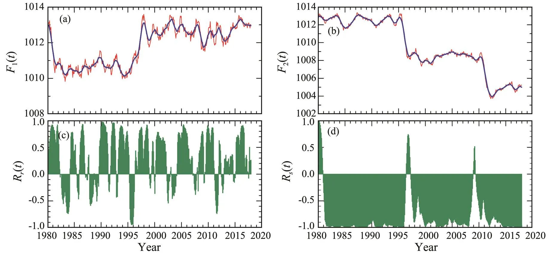
Fig.7 Running correlation dominated by low frequency. (a), Monthly air pressure (unit: hPa) in Beijing (red line) and the local mean (blue line); (b), Monthly air pressure (unit: hPa) in Guangzhou (red line) and the local mean (blue line); (c), LRCC Rr(t); (d), SRCC Rs(t). The monthly air pressure data are obtained from the China Meteorological Data Service Center.

Fig.8 Running correlation of surface air temperatures in Beijing and New York. (a), Surface air temperature (unit: ℃) with a 12-point average in Beijing (red line) and the local mean (blue line); (b), Surface air temperature (unit: ℃) with a 12-point average in New York (red line) and the local mean (blue line); (c), LRCC Rr(t); (d), SRCC Rs(t). The surface air temperature data are obtained from NCEP/NCAR Reanalysis 1.

Therefore, LRCC only reflects the correlation between high-frequency signals, whereas SRCC reflects the correlation of both high- and low-frequency signals. In parti- cular, if the correlation of phenomena with low-frequency variations or long-term trends is to be studied, SRCC is the inevitable choice.

6 Discussion and Conclusions

A running correlation coefficient (RCC) is calculated by moving the time window to study temporal variations in the correlations of two time series. The local running correlation coefficient (LRCC) is obtained by the direct application of the general definition of a correlation coefficient to the data within a time window. However, LRCC only reflects the correlation between two anomalies with- in the time window and fails to reflect the contributions of two varying means. Thus, a new method called synthe- tic running correlation coefficient (SRCC) was proposed by Zhao. (2018), which is calculated using the means of all data (global means) instead of the varying local means. SRCC reflects the correlation between varying ano- malies and varying means. However, as a recently proposed method, SRCC lacks the support of mathematical theory. In the present study, the validity of SRCC is de- monstrated theoretically by considering the comparability of RCC values in different time windows.

RCC is only meaningful when its values at different times can be compared. Thus, a pair of constants must be determined prior to the actual calculation as the standard for comparison. The unique standard quantities are demonstrated to be the global means. This result indicates that SRCCs of different time windows are comparable, but LRCCs are not. Comparability may also be expressed in the-geometric space of the two data series. The cross points of the fitted lines of LRCC at different times are found at different positions; by contrast, the cross points of SRCC are located at the same position. Therefore, the magnitudes of SRCC at different time windows are comparable, whereas those of LRCC are not.

In this study, the relationship between LRCC and SRCCwas derived by statistical methods, and SRCC was obtained by adding a constraint condition to the LRCC algorithm. Specifically, the cross points of the regression lines must pass through the center of all data represented by the global means in the geometric space. This constraint condition provides the mathematical basis of the comparison standards. Thus, SRCC is proven to be the unique RCC satisfying the comparability criterion.

When the temporal fluctuations are divided into high- frequency (., periods shorter than the time window) and low-frequency (., periods longer than the time window) signals, some examples show that LRCC only reflects the correlation of high-frequency signals. By contrast, SRCC reflects the correlation of both high and low frequencies.

Our findings do not mean that previous results obtained using LRCC are questionable. Many studies have focused on the correlation between seasonal and sub-seasonal signals, which are high-frequency variations, and LRCC is, in fact, a good measure of the relevant correlation. Ne- vertheless, if the correlation of phenomena with low-fre- quency variations or long-term trends is to be studied, SRCC is the inevitable choice because it provides the complete information of the running correlation between various periods.

More importantly, SRCC embodies the physical fact that any piece of data is a part of the whole dataset. The global means are simply parameters that include the information of the whole data. SRCC establishes the connection between local and global variations via the global means. Therefore, SRCC is the correct approach to calculate RCC.

The dependence of SRCC on global means gives rise to a unique feature of SRCC. Alterations in a data domain result in changes in the global mean. Thus, SRCC varies for different data lengths even if the same data series are used.

Acknowledgements

This study was supported by the National Natural Science Foundation of China (Nos. 41976022, 41941012), andthe Major Scientific and Technological Innovation Projectsof Shandong Province (No. 2018SDKJ0104-1).

Brown, J. R., Hope, P., Gergis, J., and Henley, B. J., 2016. ENSO teleconnections with Australian rainfall in coupled model simulations of the last millennium., 47 (1-2): 79- 93, DOI: http://dx.doi.org/10.1007/s00382-015-2824-6.

Burdun, G. D., and Markov, B. N., 1972.. Izd-vo Standartov, Moscow, 196-206.

Elias, A. G., and Zossi de Artigas, M., 2003. A search for an association between the equatorial stratospheric QBO and solar UV irradiance., 30: 1841.

Francis, J. A., and Vavrus, S. J., 2012. Evidence linking Arctic amplification to extreme weather in mid-latitudes., 39: L06801, DOI: 10.1029/2012GL051 000.

Galton, F., 1888. Correlations and their measurement, chiefly from anthropometric data., 45: 135-145.

Geng, X., Zhang, W., Jin, F. F., and Stuecker, M. F., 2018. A new method for interpreting nonstationary running correlations and its application to the ENSO-EAWM relationship., 45: 327-334.

Huybrechs, D., 2010. On the Fourier extension of non-periodic functions., 47 (6): 4326- 4355.

Hynčica, M., and Huth, R., 2020. Griddedstation temperatures: Time evolution of relationships with atmospheric circulation., 125: e2020JD033254, https://doi.org/10.1029/2020JD033254.

Ji, X. P., and Zhao, J. P., 2019. Transition periods between sea ice concentration and sea surface air temperature in the Arcticrevealed by an abnormal running correlation., 18 (3): 633-642, DOI: 10.1007/s11802- 019-3909-3.

Kodera, K., 1993. Quasi-decadal modulation of the influence of the equatorial quasi-biennial oscillation on the north polar stratospheric temperatures.,98: 7245-7250.

Kuznets, S., 1928. On moving correlation of time sequences., 23 (162): 121- 136.

Merrington, M., Blundell, B., Burrough, S., Golden, J., and Ho- garth, J., 1983. A list of the papers and correspondence of Karl Pearson (1857–1936). Publications Office, University College London.

Pearson, E. S., 1938.. Cambridge University Press, Cambridge, 193-257.

Pearson, K., 1896. Mathematical contributions to the theory of evolution.–On a form of spurious correlation which may arise when indices are used in the measurement of organs., 60 (3): 489-498.

Salby, M., Callaghan, P., and Shea, D., 1997. Interdependence of the tropical and extratropical QBO: Relationship to the solar cyclea biennial oscillation in the stratosphere., 102 (D25): 29789- 29798.

Schmid, J., 1947. The relationship between the coefficient of cor- relation and the angle included between regression lines., 41 (4): 311-313.

Soukhearev, B., 1997. The sunspot cycle, the QBO, and the total ozone over northeastern Europe: A connection through the dy- namics of stratospheric circulation., 15: 1595-1603.

Turner, T. E., Swindles, G. T., Charman, D. J., Langdon, P. G., Morris, P. J., Booth, R. K., Parry, L. E., and Nichols, J. E., 2016. Solar cycles or random processes? Evaluating solar variability in Holocene climate records., 6: 23961, https://doi.org/10.1038/srep23961.

Varotsou, E., Jochumsen, K., Serra, N., Kieke, D., and Schneider, L., 2015. Interannual transport variability of upper Labrador Sea water at Flemish Cap., 120: 5074-5089.

Woods, J. W., and Oneil, S. D., 1986. Subband coding of images., 34: 1278-1288.

Zhao, J. P., and Huang, D. J., 2001. Mirror extending and circular spline function for empirical mode decomposition method., 2 (3): 247-252.

Zhao, J. P., and Drinkwater, K., 2014. Multiyear variation of the main heat flux components in the four basins of Nordic Seas., 44 (10): 9-19 (in Chinese with English abstract).

Zhao, J. P., Cao, Y., and Shi, J. X., 2006. Core region of Arctic oscillation and the main atmospheric events impact on the Arctic., 33: L22708.

Zhao J. P., Cao, Y., and Wang, X., 2018. The physical significance of the synthetic running correlation coefficient and its applications in oceanic and atmospheric studies., 17 (3): 451-460.

Zhao, J. P., Drinkwater, K., and Wang, X., 2019. Positive and negative feedbacks related to the Arctic oscillation revealed byair-sea heat fluxes., 71 (1): 1-21.

November 5, 2020;

January 20, 2021;

January 29, 2021

© Ocean University of China, Science Press and Springer-Verlag GmbH Germany 2021

. Tel: 0086-532-66782096 E-mail: jpzhao@ouc.edu.cn

(Edited by Chen Wenwen)