Xiao-Yi Chen(陈晓义), Ya-Xuan Duan(段亚轩), Bin-Bin Xiang(项斌斌),Ming Li(李铭), and Zheng-Shang Da(达争尚)

1The Advanced Optical Instrument Research Department,Xi’an Institute of Optics and Precision Mechanics,

Chinese Academy of Sciences,Xi’an 710119,China

2University of Chinese Academy of Sciences,Beijing 100049,China

3Xinjiang Astronomical Observatory,Chinese Academy of Sciences,Urumqi 830011,China

Keywords: angular spectrum,diffraction,Fourier optics and signal process

1. Introduction

Digital simulation of scalar diffraction is widely used for studies like phase retrieval,[1-6]digital holography,[7,8]optical information security,[9]and computational imaging.[10,11]These simulations of diffraction are usually based on the wellknown scalar diffraction theories. For parallel planes,[12]there are mainly three methods of field propagation called the single Fourier-transform-based Fresnel method(SFT-FR),the convolution-based Fresnel method (CV-FR), and the AS method respectively. The SFT-FR has the fastest speed, but the sampling interval is proportional to the propagation distance. To control the sampling interval, the multi-step Fresnel method[13-15]and shifted Fresnel method (shift-FR)[16]have been proposed. The CV-FR and AS are all convolutionbased methods,so the sampling window and the sampling interval in the input plane are the same as those in the output plane. Compared with CV-FR,AS is more accurate as it is directly derived from Rayleigh-Sommerfeld diffraction theory without approximation.[17,18]But the sampling problem in the transfer function makes that AS only accurate for quite near field. However,the long-distance propagation often occurs in some applications such as wavefront detection,computational holography,and antenna detection.

There are two effective methods to achieve long-distance propagation based on AS. One is adding a wide calculation window(zero-padding)in the input plane, which will lead to large amount of calculation. The other is BLAS[19]method,in which the transfer function is truncated to a proper bandwidth.The aliasing transfer function components are forced to be zeros and only the non-aliasing transfer function components are used. It has been shown that the effective non-aliasing bandwidth of the transfer function would decrease rapidly when the propagation distance increases. So, the accuracy of BLAS in inverse calculation from the output plane to the input plane decreases as the propagation distance increases.[19,20]Therefore,the application of BLAS in iterative phase retrieval technology is limited.

In this paper, a modified scaling angular spectrum(MSAS)method for long-distance propagation is proposed. It consists of two parts, the scaling calculation and the choice of calculation window. Firstly, a scaling factor is introduced so that the sampling interval of input plane can be defined independently. And by applying the Bluestein substitution,the discrete Fourier transform can be used even if the sampling intervals of input plane are different from that of output plane.[21-24]The calculation speed of MSAS is fast because it is based on a linear convolution which can be evaluated by fast Fourier transform (FFT) effectively. Then the most suitable size of the calculation window is selected so that the numerical calculation in long-distance propagation runs efficiently. Unlike the truncation of the transfer function in BLAS method,the proposed method can also be accurately calculated in the inverse calculation.

The rest of this paper is arranged as follows:In Section 2,the principle of traditional long-distance propagation is introduced in details. Section 3 discusses the MSAS proposed in this paper and explains it from three parts: the scaling calculation of MSAS,the calculation window of MSAS,and computational complexity. In Section 4,MSAS is compared with other methods when used for numerical calculation in longdistance propagation. In Section 5, the simulations are verified through experiments. Finally, in Section 6, conclusions are drawn.

2. The principle of the traditional long-distance propagation

In the scalar diffraction theory, the accurate diffraction formula is the Rayleigh-Sommerfeld diffraction integral. It is always converted into a convolution form which is also called the AS formula

where z is the propagation distance, (x0,y0) and U0(x0,y0,0)are the coordinates and the light field of input plane,(x,y)and U(x,y,z)are the coordinates and the light field of output plane,F and F−1represent the Fourier transform and inverse Fourier transform,respectively. H(u,v,z)is the transfer function,

where λ is the wavelength,u and v are the Fourier frequencies in x and y directions,respectively.

The calculation of AS is based on the discrete Fourier transform (DFT) which only describes the discrete periodic function. As shown in Fig.1, the sampling of the input field would result in the generation of modulated and translated replicas in periodic locations of the input plane. To avoid the aliasing error, the discrete calculation of Eq. (1) need to meet Nyquist sampling theorem. So the discrete transfer function’s sampling rate of change is less than or equal to π when m=M/2,n=N/2,we obtain[25]

where m = −M/2,−M/2 + 1,...,M/2−1 and n =−N/2,−N/2+1,...,N/2−1, M and N are the sampling numbers in the x0and y0directions, Δx0and Δy0are the sampling intervals in the x0and y0directions, respectively.Therefore,the propagation distance z need to satisfy

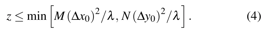
In AS, the sampling intervals of the input plane are equal to the sampling intervals of the output plane. Meanwhile, the sampling intervals of the output plane are determined by the pixel sizes of detector. Once the pixel sizes of the detector(Δx,Δy)are determined,the sampling intervals of input plane(Δx0=Δx, Δy0=Δy) are also determined accordingly. According to Eq. (4), the propagation distance is restricted to a limited value.

Fig.1. Replicas of the physical window in the input plane.

Another way is to truncate the transfer function to a limited bandwidth, which is called BLAS. The expression of its transfer function is[19]

where ulimand vlimare

where Δu = 1/[2(MΔy0)], Δv = 1/[2(NΔy0)]. Although BLAS increases the propagation distance, high-frequency information is lost due to the limited bandwidth in the frequency domain and the accuracy in inverse calculation is also limited.

3. Modified scaling angular spectrum propagation

3.1. Scaling calculation of MSAS

From Eq. (4), the propagation distance is also related to the sampling intervals in the input plane. As the sampling intervals increase,the propagation distance increases. However,the sampling intervals between the input plane and the output plane are equal in traditional long-distance propagation.Therefore, MSAS consists of two parts: the scaling calculation and the selection of calculation window. One is to freely define the sampling interval of the input plane, and the other is to select the most suitable size of calculation window for long-distance propagation.

MSAS is derived from AS, and the coordinate system used in formulas is shown in Fig.2. P and Q are the sampling numbers of calculation window in the x0and y0directions,respectively. R and T are the sampling points of the input field in the x0and y0directions, respectively. The discrete Fourier transform of the input plane A(up,vq,0)can be expressed as

where x0p= pΔx0,y0q=qΔy0,up= pΔu,and vp=qΔv. So,the diffraction field of output plane is

where

A(up,vq,z)=A(up,vq,0)H(up,vq,z)

is discrete Fourier transform of the output plane, xr= rΔx,yt=tΔy. Δx and Δy are the sampling intervals of output plane in x and y directions,respectively. We cannot directly use the inverse discrete Fourier transform to calculate the summation of Eq. (9) because of the differences of the sample intervals and sampling numbers in the input and output planes(P/=R,Q/=T,Δx/=Δx0,Δy/=Δy0). To solve this problem,a scaling factor h is firstly introduced into Eq.(9)as

Additionally, the term (2hupxr+2hvqyt) can be converted to the following expression:

which is known as Bluestein substitution.[22]Then the summation process in Eq.(10)is converted into a discrete convolution

where

the star operator “∗” denotes the discrete convolution operation.

Fig.2. Geometry of the propagation model between input plane and output plane.

Due to Δu′=Δx, Δv′=Δy, the discrete convolution can also be effectively evaluated by FFT. By Eq. (11), we can choose the independent sampling intervals in the input plane.Meanwhile, the sampling numbers between the input plane and the output plane need not be the same because of the linear convolution.As for the inverse propagation,just let z equal−z and exchange the position of Δx0and Δx,Δy0and Δy,the calculation formula is still the same as Eq.(11).

The sampling intervals of input plane can be smaller than, equal to, or larger than the sampling intervals of output plane.However,Δx0＞Δx and Δy0＞Δy are required for longdistance propagation in MSAS to reduce the sampling numbers of calculation window. According to Eq. (4), when the distance is constant, the sampling intervals of the input plane must meet the following condition:

3.2. Calculation window of MSAS

Similarly, a suitable calculation window should be selected in MSAS to make sure that the sampling in the frequency domain is effective for long-distance propagation. In MSAS,increasing the sampling interval in the input plane will reduce the sampling number of the calculation window,so the amount of calculation will be greatly reduced. Taking x0and x axes as examples,y0and y axes can be analogical.

Firstly, the range of sampling frequency in the transfer function within which no aliasing error occurs must be determined by Eq.(7).[19]The required sampling interval Δu of frequency domain is

Therefore, according to Eqs.(7)and(13), the size of the calculation window is

Secondly,to convert a circular convolution to a linear convolution, the input field needs to be doubled both in x and y axes.[21,22]

In addition, FFT will broaden the spectrum of input field. In order to ensure that the aliasing spectrum will not overflow into the output plane,the size of calculation window needs to satisfy[26]

where Wx=RΔx0and Sx=RΔx are the size of input field and observation window in x0and x directions,respectively.

In summary,the calculation window Lxwill be the maximum of L1x, L2xand L3xfor meeting all these requirements from Eqs. (14)-(16). P can be obtained by Lx, Δx0, and Q is analogical.

As shown in Fig.3, the highest spatial frequency observed at the upper end of observation window may be given by the field coming from the lower end of the input field. Therefore, the minimum bandwidth of the spectrum which is needed for exact numerical propagation is

After adding the calculation window by Eq. (17), the maximum bandwidth which MSAS can be correctly sampled is[19,27]

If umax＜uneed, the input field loses a part of the frequency band necessary for exact diffraction. Therefore, for an accurate sample,the relation between umaxand uneedis

From Eqs. (18)and(19),we know the following two points.

(i)if L=max(L1,L2,L3)=L3,umax=uneed;

(ii)if L=max(L1,L2,L3)=L1or L2,umax＞uneed.

So equation(20)is always satisfied.

Fig.3. A model for minimum bandwidth required for exact numerical propagation.

Figure 4 shows a sampled transfer function of AS,where the parameters are M = 1024, z = 50MΔx, λ = 635 nm,Δx=2λ, and Δx0=2λ. Only the real part of transfer function is depicted in the sampling interval Δu=1/MΔx0of AS.Because the transfer function is a kind of chirp function, an aliasing error is introduced in the sampled transfer function as shown in Fig.4. With MSAS method, Δx0increases to 10λ and the calculation window is determined by Eq. (17). Then the maximum bandwidth umaxcan be calculated by Eq. (19).As a result,the aliasing error is removed.

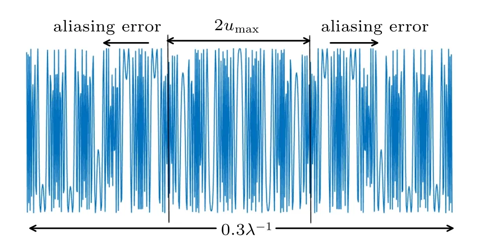
Fig.4. Example of a sampled transfer function of AS and MSAS.

3.3. Computational complexity

Both the AS and PAS use two Fourier transforms. The computational complexity can be calculated by the following formulas:

In MSAS,one FFT calculations and one FFT-based linear convolution are used,so the computational complexity is

Under long-distance propagation, the sampling number required by MSAS is less than that required by PAS(M ≤R ＜P ＜MPAS, N ≤T ＜Q ＜NPAS), so the computational complexity is low(CAS＜CMSAS＜CPAS)and the calculation speed is faster than PAS. Moreover, as the propagation distance increases, more sampling number is required for PAS and the advantage of MSAS is more significant.

4. Simulation

In order to prove the effectiveness of MSAS, we performed the following simulation and compared it with AS,PAS, and BLAS. The parameters of simulation are as follows: the detector pixel size is Δx=Δy=7.4µm, the wavelength is λ = 635 nm, the width of the square aperture is 0.5 mm, the sampling number of the object plane is chosen to be M×N =200×200 to convert a circular convolution to a linear convolution.[21,22]

In AS, BLAS, and PAS, the sampling interval of input plane is the same as that of output plane.The sampling number in AS does not change with the propagation distance,which is always MAS×NAS=200×200. However,the sampling number of BLAS is MBLAS×NBLAS= 400×400 and the sampling number of PAS(MPASand NPAS)increases according to Eq.(5).

Fig.5. The minimum sampling number in the diffraction area and the sampling interval of MSAS changes with propagation distance. (a) The minimum sampling number in the diffraction area changes with propagation distance;(b)the sampling interval of MSAS changes with propagation distance.

As the distance increases, the diffractive propagation is divergent. In MSAS, the minimum sampling numbers (R,T = R) of diffractive area required for diffraction propagation are determined as shown in Fig.5(a) according to different diffraction distances. The sampling intervals under different propagation distances in the input plane are determined by the minimum sampling numbers and Eq.(12)as shown in Fig.5(b). Then the minimum sampling numbers and sampling intervals determine the sampling number(P,P=Q)of calculation window.

Fig.6. Comparison of AS, BLAS, PAS, and MSAS. (a) The SNR of AS,BLAS,PAS,and MSAS changes with propagation distance;(b)the calculation time of AS,BLAS,PAS,and MSAS changes with propagation distance;(c)the inset clearly shows calculation time of AS,BLAS,and MSAS when the distance from 0 mm to 500 mm.

Accuracy is evaluated by SNR of the diffraction intensity:[28]

where I(x,y) is the calculated diffraction intensity of output plane obtained by AS, BLAS, PAS or MSAS. Irig(x,y)stands for the diffraction intensity on the output plane obtained by the accurate Gauss-quadrature numerical integral(NI)method,[29,30]where α is introduced as follows:

As shown in Fig.6(a), the SNR calculated by BLAS and AS gradually decreases when the distance is larger than 27 mm and 418 mm respectively.BLAS and AS no longer have an advantage in the long-distance propagation. However,the SNRs of PAS and MSAS tend to increase as the distance increases.PAS and MSAS have very good SNR,but the running speed of MSAS is faster than PAS as the propagation distance increases which is shown in Fig.6(b). The running speed is consistent with the computational complexity described in Subsection 3.3. In the simulation,MATLAB(Version R2016b,Math Works, Natick, Massachusetts) installed in a 3.40-GHz central processing unit(Intel core i7-6700)and 8 GB of randomaccess memory desktop computer was used for calculation.

Taking z1=100 mm and z2=500 mm as examples,the two-dimensional (2D) diffraction intensity, one-dimensional(1D) amplitude, and phase of AS, BLAS, MSAS, PAS, and NI are shown in Fig.7. When the distance is z1=100 mm,the amplitude and phase calculated by AS are already incorrect as shown in Fig.7(a). However,the amplitude and phase of BLAS, PAS, and MSAS are all consistent with that of NI.When the distance is z2=500 mm, BLAS and AS cannot be calculated accurately as shown in Fig.7(b). But both MSAS and PAS can be calculated accurately like NI,and MSAS runs faster than PAS.

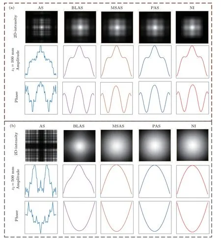
Fig.7. The 2D-diffraction intensity,1D-amplitude,and phase using AS,BLAS,MSAS,PAS,and NI in z1=100 mm and z2=500 mm,respectively.(a)z1=100 mm;(b)z2=500 mm.

The intensities calculated inversely by MSAS and BLAS under the distances of z1=100 mm and z2=500 mm are given in Fig.8. Due to the limitation of the bandwidth in the transfer function,the accuracy of inverse calculation in BLAS decreases with the increase of propagation distance as shown in Figs.8(a),8(b),8(a1),and 8(b1). The application of BLAS in the iterative phase retrieval technology is limited. But MSAS is not restricted to inverse calculation as shown in Figs.8(c),8(d),8(c1),and 8(d1).

Fig.8. The 2D-intensity and 1D-intensity using the inverse calculation of BLAS and MSAS under z1 =100 mm and z2 =500 mm. BLAS: (a) the inverse result in z1=100 mm,(a1)center section view of panel(a);(b)the inverse result in z2=500 mm,(b1)center section view of panel(b);MSAS:(c)the inverse result in z1=100 mm,(c1)center section view of panel(c);(d)the inverse result in z2=500 mm,(d1)center section view of panel(d).

5. Experiment

The experimental setup is shown in Fig.9. The laser with a wavelength λ =635 nm goes through the collimating lens and the pinhole,getting to the CCD.The diameter of the pinhole is 0.5 mm, the pixel size of CCD is Δx=Δy=7.4 µm with a total number of pixels is 1600×1200. The PV of wavefront error is 0.13λ (the caliber is φ =6 mm)so that the wavefront in the pinhole can be approximated as a plane wave. The distances between the pinhole and CCD are z1=113 mm and z2=520 mm,respectively.

Fig.9. Experimental setup.

When the distance is z1=113 mm,the sampling number in the pinhole plane is MPAS×NPAS=1310×1310 by using PAS. Using MSAS, the sampling interval of pinhole plane is Δx0=Δy0=16.7µm and the sampling number of calculation window is P×Q=512×512. Similarly, when the distance is z2=520 mm, the sampling number using PAS in the pinhole plane is MPAS×NPAS=6030×6030. Using MSAS,the sampling interval of pinhole plane is Δx0=Δy0=18.1 µm and the sampling number of calculation window is P×Q=2016×2016.

Figure 10 shows the diffractive spots of PAS,MSAS,and experiment. The one-dimensional cross-sectional views of MSAS and experiment along the center are shown in Fig.11.In order to further prove the agreements between simulation by MSAS and experiment, the correlation coefficient c is defined

From Figs.10(b)and 10(e),there is no periodic artifacts appear in the diffraction spots calculated by MSAS under two distances. Either in Fig.10 or Fig.11, MSAS is also highly consistent with the experimental results. And the correlation coefficients of the two in z1=113 mm and z2=520 mm are c1=0.9502 and c2=0.9992,respectively.As the propagation distance increases, the correlation coefficients increase because the influence of wavefront aberration is getting smaller.And the calculation time of PAS is about 3.93×and 5.77×of MSAS in z1=113 mm and z2=520 mm,respectively.Therefore, for long-distance propagation, the calculation of MSAS is accurate and fast.

Fig.10. The diffractive spots of PAS, MSAS, and experiment. Top row: z1 =113 mm, (a) calculated by PAS, (b) calculated by MSAS, (c)experiment;bottom row: z2=520 mm,(d)calculated by PAS,(e)calculated by MSAS,(f)experiment.

Fig.11. One-dimensional cross-sectional views of MSAS and experiment along the center: (a)z1=113 mm,(b)z2=520 mm.

6. Conclusion

In conclusion, a modified scaling angular spectrum(MSAS)method to solve the problem in AS for long-distance propagation is proposed. The method consists of two parts,the scaling calculation and the selection of calculation window. The former is used to freely define the sampling intervals of the input and output planes. The latter is to ensure that MSAS is calculated accurately for the long-distance propagation. It is indicated from the simulation and experiment that MSAS is highly consistent with NI and experimental results,and the calculation speed is faster than PAS.Meanwhile,MSAS does not limit bandwidth in the frequency domain like BLAS, so its accuracy in inverse calculation is much higher than BLAS. Both simulation and experiment prove the correctness of MSAS and it has a great prospect for application in iterative phase retrieval.