Bing-Lan Wu(吴冰兰), Qiang Wei(魏强), Zhi-Qiang Zhang(张智强),†, and Hua Jiang(江华),3,‡

1School of Physics and Technology,Soochow University,Suzhou 215006,China

2State Key Laboratory of Quantum Optics and Quantum Optics Devices,Institute of Laser Spectroscopy,Shanxi University,Taiyuan 030006,China

3Institute for Advanced Study,Soochow University,Suzhou 215006,China

Keywords: disorder effect,pseudo-magnetic field,strain,transport properties

1. Introduction

Over the past decades, the pseudo-magnetic field (PMF)attracts lots of attention due to the synthetic gauge field induced by the mechanical strain in materials,[1-4]which provides a new way of tailoring their electronic properties.[5-15]In graphene,for example,inhomogeneous strain can modulate the coordinate of Dirac cones which initially located at highsymmetry points K and K′.[1,2]Such inhomogeneous straininduced pseudo-gauge field Asenters into the effective Dirac Hamiltonian H=vfσ·p by replacing the mechanical momentum p with the generalized momentum p±eAs,where±denotes the K and K′valleys,respectively. In experiments,various inhomogeneous strained structures have been realized for graphene,[16-23]and the related PMF can reach up to hundreds of Teslas.[24,25]

The huge field strength also promotes many experimental groups to explore the PMF in artificial graphene systems.[26-28]Among them,the realization of PMF in phonon crystals is an important progress in recent years.[29-32]Especially, PMF induced Landau levels (LLs) and edge states are successfully achieved in such a system.[32]It is natural to ask whether these two states pose the similar transport properties to those in magnetic fields (MFs). As is known, in quantum Hall effect,the edge states introduced by the MFs(U(1)gauge field)are robust against disorder,[2,33-36]while the corresponding LLs are localized. However,the edge states and the LLs in PMF[29,37-43]should be different,since the time-reversal symmetry ensures that the effective PMF of K valley is opposite to that of K′. Therefore, the influence of disorder to states in PMF should be addressed.

In this paper,we study the transport properties of states in PMF.First,we construct an inhomogeneous strained graphene structure in which an uniform PMF is obtained. Then, the influence of disorder to LLs and edge states is numerically calculated. We find that the edge states induced by PMF are fragile to disorder. Furthermore,the dispersion of LL(except the zeroth LL) is tilted. It acts as one-dimensional channel inside the bulk, and disorder can also cause strong backscattering.We also find that the backscattering for both edge states and LL channels originating from PMF can be suppressed by an external MF,[40,44]because the spatial overlap between counter-propagating channels protected by time-reversal symmetry will be lifted. The above behaviors have the potential application in mesoscopic devices.

2. Strained graphene model and corresponding spectra

We consider a model with inhomogeneous strained graphene structure, as shown in Fig.1(a). The tight-binding Hamiltonian reads[1,2]

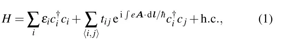
To simulate the inhomogeneous stain-induced PMF,the hopping strength tijis simply classified into two categories.[40,47]First,the inhomogeneous strain-induced hopping in the vertical direction(y)is a linear function of the position y,

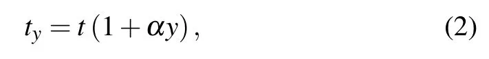
in which α (in units of a−1, a is the lattice constant) is the parameter that characterizes the degree of strain. t is the energy unit. A typical distribution of tyis plotted in Fig.1(b). It shows the hopping strength marked in Fig.1(a)by red dashed ellipses. Second,the hopping strength in the other two directions remains a constant tij=t(see Appendix A).The effective Hamiltonian for K valley is written as[1]

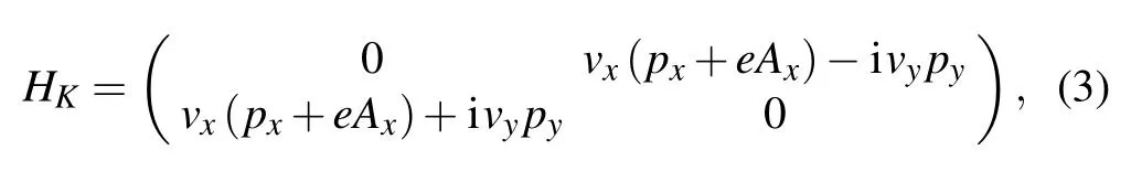
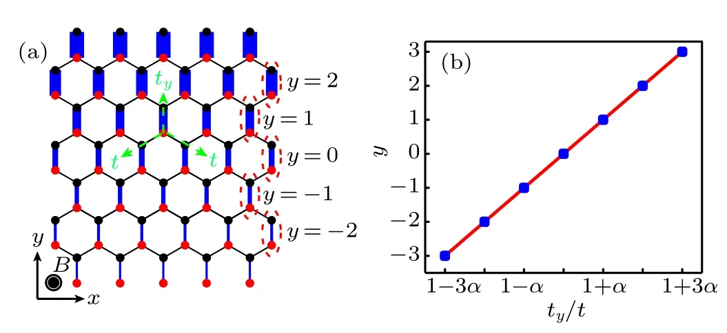
Fig.1. (a)A realization of PMF in graphene. It is achieved by adjusting the hopping along y direction. The MF is along z direction,and the width of the solid lines implies the hopping strength. The dashed green arrows show the vertical hopping ty and the rest of the hopping t. (b)A typical plot of ty versus y for(a).

3. Transport properties of edge states of strained graphene

In common view,topological edge states should be robust against disorder and lead to disspationless transport,[51-56]e.g.,QH and QSH.Very recently,such guideline more or less motivates the discovery of ‘QH’ induced by PMF. Thus, we first investigate the transport properties of edge states under PMF in this section.

Figures 2(c)and 2(d)show the distribution of edge states with Ef=0.016t [see the green and black dots in Figs. 2(a)and 2(b)]. Different from the edge states of QH systems, the counter-propagating states under PMF only exist around the Ny=202 boundary,being consistent with previous studies.[29]It is noteworthy that the quality of edge states in this strained graphene depends on the ribbon width Nyand strain parameters α (see Appendix C). Since the spatial overlap will enhance backscattering between the counter-propagating states,one can anticipate that edge states in PMF would be fragile to disorder. Thus, we study the variation of differential conductance G for edge states under disorder. For simplicity,the Fermi energy is fixed at Ef=0.016t with φ =0 (i.e., MF is absent),where only the edge states exist[see Fig.2(a)]. When the disorder concentrates on the upper region of the sample[see Fig.3(a)],we find that G decreases sharply even for weak disorder[see Fig.3(c)]. In contrast,if disorder locates on the area without edge states, the G =e2/h plateau exists when W ＜t [see Figs.3(b)and 3(d)]. The behavior of G also suggests that the counter-propagating edge states under PMF distinguish from the helical edge states in QSH, since the latter are robust against nonmagnetic disorder.

We also find that the external magnetic field will significantly redistribute the edge states when φ is large enough.For example, we plot the band structure in Fig.2(b) with φ =0.012,where the counter-propagating edge states become separated in space[see Figs.2(c)and 2(d)]. The redistributed channels are robust under disorder,which implies that the external magnetic field can eliminate the backscattering of the sample. If the edge states induced by PMF are destroyed by disorder,the external magnetic field will rebuild the quantized differential conductance G. As shown in Figs. 3(c) and 3(d),G increases with the increase of φ and reaches the quantized value e2/h again at φ =0.016. In practical application,since disorder inevitably exists and edge channels induced by PMF can be destroyed even under weak disorder (W ≪t),a switch device could be achieved by adjusting the magnetic field strength in a sample with PMF.

Fig.2. (a)and(b)The energy spectra with the same strain parameters α =0.015,and the MFs are φ =0 and φ =0.012,respectively. (c)and(d)The probability density distributions for the edge states marked with black and green circles in panels(a)and(b).

Fig.3.(a)and(b)Schematic representation of two-terminal device(width Ny=202,length Nx=100),in which the violet region is disordered.The counter-propagating edge states are labeled with black and red arrows,where the left-moving edge states with and without φ are represented by solid red arrows and dotted red arrows,respectively. (c)and(d)Two-terminal differential conductance G versus disorder strength W for the devices shown in(a)and(b),respectively. The Fermi energy is fixed at Ef=0.016t.

4. Transport properties of LLs of strained graphene

Interestingly, compared with the localized LLs in QHE,we find that LLs of strained graphene impose unique transport properties. Due to the uniform Bs, the energy spectrum in strained graphene is also quantized into discrete LLs

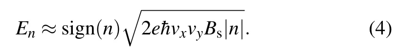
Here,n is the LL index. Significantly,if n/= 0,the LLs are no longer flat as it would be in an external MF,and thus it is more appropriate to call them pseudo-Landau levels(see Appendix D).For better comparison,we will still call them Landau levels(LLs). This is because both vx,vyand eigen-wavefunction[57]

Figure 4(b) plots the spatial distribution of typical states for n=−1 LL with Ef=−0.173t and φ =0 [i.e., the red and gray circles in Fig.4(a)]. When MF is absent, the red and gray curves(corresponding to wavefunctions of forwarding LL and its counterpart) in Fig.4(b) overlap due to the time-reversal symmetry, and the center of the wavefunction is located around Ny=100. The effect of disorder on these states is also investigated. When Anderson disorder is applied to all areas of the device (i.e., both areas of A and B in Fig.4(c)),differential conductance G decreases to zero for W ＞3t (see the red line in Fig.4(d)), meaning all the states are localized by disorder. Then, we remove disorder in the range Ny∈[50,150](i.e.,yellow region A in Fig.4(c)). G for such condition holds e2/h plateau even when W ＞3t [see the black line in Fig.4(d)]. These results imply that one channel still exists. According to Fig.4(b), such conducting channel is corresponding to LL states. Moreover, the conducting LLs provide a routine to realize one-dimensional channels in a twodimensional system,and one can manipulate the on/off status of these channels by adjusting the distribution of disorder.

Fig.4. (a)Energy spectrum of the strained graphene ribbon with α =0.015 and Ny=202. The system holds time-reversal symmetry since the real MF φ =0. (b)The typical probability density distribution of counter-propagating bulk n=−1 LL states marked with the gray and red circles in panel(a)at Ef=−0.0173t. (c)Schematic of two-terminal device. The yellow region with width δNy=10 and two violet regions represent bulk disordered region A and edge disordered area B, respectively. (d) Differential conductance G versus disorder strength W at Ef =−0.0173t. (e) Probability density distributions|Ψ|2 versus combinations(Ny ,E)for all the bulk states in n=−1 LL.The color bar represents the probability density. (f)G for the device shown in panel(c)with the disordered region B shifting from[85,95]to[105,115]. The disorder strength is fixed to W =4t.

Although both edge states and LL states in PMF are onedimensional channels, their energy dependent behaviors are totally different. The spatial distribution of edge states (LL states)is insensitive(sensitive)to E. To deeply understand the LL states,we present their distribution of wavefunction versus Nyand energy E for the n=−1 LL.As shown in Fig.4(e),all the states of the LL are on the bulk of the sample. Also, the center of the wavefunction shifts almost linearly in space with an increase of E.These results are consistent with Eqs.(4)and(5)that the LLs(n/=0)are y(Ny)dependent.According to the above LLs behaviors,one can filter corresponding conducting channels for particular energy E region through engineering the disorder distribution. As shown in Fig.4(c),we put disorder only in region A.The differential conductance G decreases by e2/h[see Fig.4(f)],meaning that one of the bulk LL channels is filtered by the disorder. Moreover, the filtered energy region shifts to the lower energy as the disordered region A moves from[85,95]to[105,115]. It agrees with the distribution of wavefunction for LLs[see Fig.4(e)].

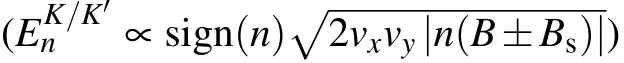
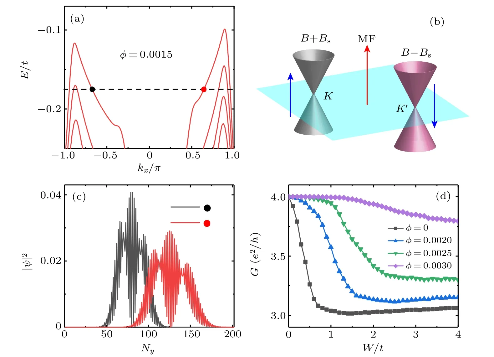
Fig.5. (a) Energy spectrum of the strained graphene ribbon with α =0.015, Ny =202, and the external magnetic field φ =0.0015. (b)Schematic diagram of effective magnetic field in K and K′ valleys. The blue and red arrows represent the directions of the PMF and MF,respectively. (c)The probability density distribution of counter-propagating n=−1 LL states at Ef =−0.0177t (the black and red circles in panel(a)). (d)G versus disorder strength W with the disorder distributing in the range Ny ∈[105,115]for different MF φ. Other parameters are the same as those in Fig.2.

5. Conclusion

In summary, we study the transport properties of graphene states under inhomogeneous strain. We find both edge states and bulk LL states induced by pseudo-magnetic field build one-dimensional conducting channels,but they tend to be localized after the disorder is introduced. However,with the help of a real magnetic field,the suppression of backscattering recovers the conducting channels from localized LL states and edge states. Based on these results, a switching device could be realized in disordered pseudo-magnetic field graphene by adjusting the real magnetic field.

Acknowledgement

We are grateful to Chui-zhen Chen and Rui-Chun Xiao for helpful discussion.

Appendix A

When the uniaxial deformation is along an armchair direction(i.e.,the y axis in the main text),the hopping strength t1(ty),t2,t3in all three directions will change.According to the equation given in Ref.[47],the hopping strengths t2and t3can be expressed as t2=t3=(1+αy)0.12≈1+0.12αy ≈1 when assuming t1=1+αy. In order to further clarify the appropriateness of the approximation t2,3≈1,we plot the energy spectrum of strained graphene for t2,3=1 and t2,3=(1+αy)0.12in Fig.A1,and there is only little difference between the two models.Thus,our main results still hold.Besides,the hopping strength shown in our main text can be easily realized in artificial systems,[i.e.,photonic crystals,electric circuits,etc.]. In our main text,we set t2,3=1 only for simplicity.

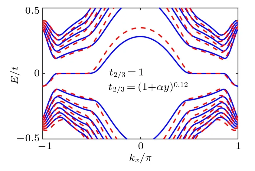
Fig.A1. Energy spectrum of the strained graphene for t2,3 =1 (blue solid line)and t2,3=(1+αy)0.12 (red dashed line).

Appendix B

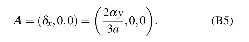
In this appendix, we present the detailed derivation of the pseudo-gauge potential A and the Fermi velocity vx,vyin strained graphene. Since the results of K′valley are similar to those of K valley,we only consider the K valley for simplicity.

Based on the tight-binding approximation, the Hamiltonian of an unstrained graphene can be written as

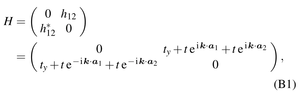
in which ty=t and

The corresponding Dirac point in K valley is sitting at

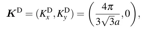
which satisfies

For the strained graphene, ty= t is replaced by ty=t(1+αy). Thus, the Dirac point K is shifted from KDto KS=KD+δ,and the follow equation still holds:

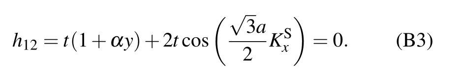
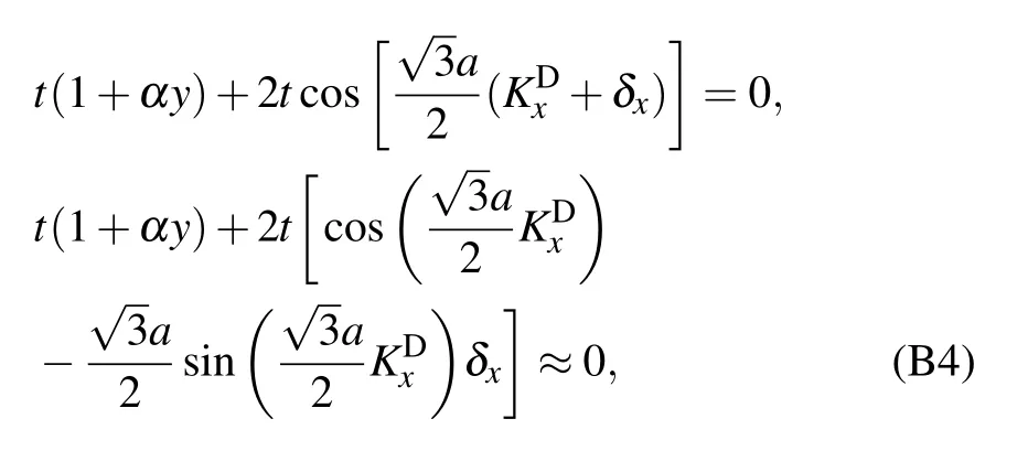
Using KS=KD+δ, equation(B3)can be rewritten around the original Dirac point KDas

To obtain the Fermi velocities vx,vy,we replace κ by KS+Δ.Then,the tight-binding Hamiltonian is given as follows:

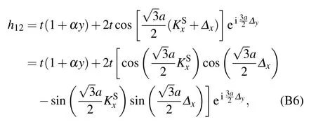
in which Δ=(Δx,Δy)is a vector between KSand κ. Moreover,

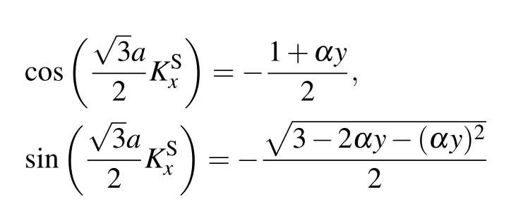
[see Eq. (B3)]. After Taylor expanding h12to the first order,we find

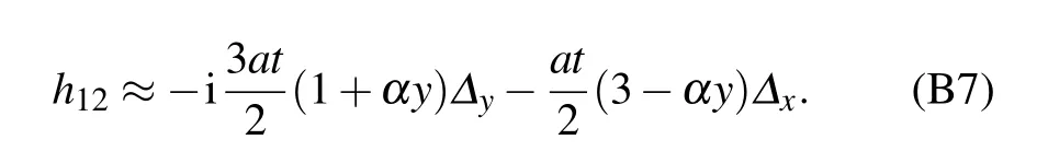
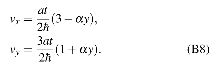
Based on Eq.(B7),the Fermi velocities are

Appendix C

In this appendix, we study the variation of the relative broadening of the edge state l/Nywith strain parameters α for two different system sizes Ny=202 and Ny=162,where l is the edge state broadening and Nyis the ribbon width.

It can be seen from Fig.C1 that the smaller the strain strength is,the wider the edge state is expanded. However,for the larger system, its relative expansion is still small. Therefore,in order to obtain high-quality edge states,a larger strain parameter is needed for systems with a smaller sample size.

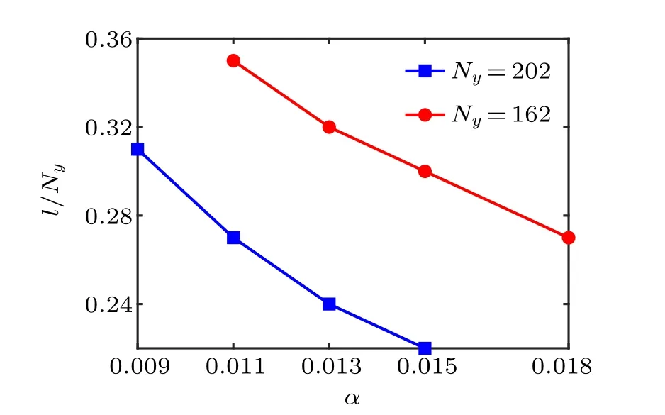
Fig.C1. The relative broadening of the edge state l/Ny for different strain parameters α,where the red and the blue lines correspond to the ribbon widths Ny=202 and Ny=162,respectively.

Appendix D

Unlike in a real magnetic field,the LLS formed in a PMF can be tilted. As shown in Fig.D1, the tilted bands (except states with zero energy)under PMF are obtained as expected,and all the states are on the bulk of the sample. Further, the corresponding edge states are also observed(see the inset near Ny=202). Thus,these bands are similar to the traditional LLs in real magnetic fields,except the tilted dispersion. It is more appropriate to call them pseudo-Landau level(PLLs).

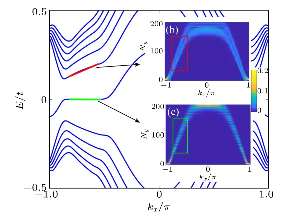
Fig.D1. (a) Energy spectrum of the strained graphene ribbon with α =0.015,Ny=202. (b)and(c)Probability density distributions versus combinations (Ny, kx) for all the states in the 1st and 0th energy levels,respectively. The states marked by the red and green lines in(a)correspond to the bulk states in the red and green boxes in(b)and(c),respectively.