SHAO Guihang, and LI Yuguo, 2), *

Numerical Simulation and Analysis of Electromagnetic Fields Induced by a Moving Ship Based on a Three-Layer Geoelectric Model

SHAO Guihang1), and LI Yuguo1), 2), *

1),,,,266100,2),,266237,

In this paper, we present a numerical simulation method of electromagnetic (EM) fields induced by a moving ship (EMFMS), which consist of both the shaft-rate EM field and the static EM field. The shaft-rate EM fields in the frequency domain are first obtained by solving the partial differential equations together with suitable boundary conditions, and then they are transformed into the time domain by using the inverse Fourier transform. Finally, the static fields are added to obtain the EM fields of a moving ship. The effects of the source current intensity and the source position on the EM fields of a moving ship are discussed in detail. A field example of EM response of a moving ship is presented and its characteristics are analyzed.

moving ship; shaft-rate EM field; static EM field; numerical simulation

1 Introduction

In order to prevent seawater corrosion, ships are often equipped with cathodic protection devices. The currents pro- duced by cathodic protection devices usually form two circuits as shown in Fig.1 (Jeffrey and Brooking, 1999). The one flowing through the ship’s propeller is modulated by the varying bearing resistance, and generates shaft-rate electromagnetic fields (Holtham., 1999). The other flowing through the ship’s coating damage point generates static electromagnetic fields (Nain., 2013). Thus, the electric and magnetic fields induced by a moving ship (EMFMS) consist of both the shaft-rate field and the sta- tic field.

The study of ship’s EM fields began in the 1960s (Zolotarevskii., 2005), and many studies on EMFMS have been conducted since then (Holmes, 2006). In these studies, however, simulation problems are often simplified. For instance, the geoelectric model is designed as an air- sea two-layer model (Sun., 2003; Lu., 2004; Liu., 2004; Zhang and Wang, 2016), in which the current source of a moving ship is assumed to be equivalent to a horizontal electric dipole (Lu., 2005; Ni., 2006), or the shaft-rate EM fields are neglected (Bao., 2011; Li., 2012). Although these simplifications can reduce the complexity of numerical simulation, they donot sufficiently simulate the real situation. Therefore, three types of problems can be caused by the simplifications. Firstly, in shallow water areas, the seafloor sediment layer has a great influence on the EM responses of a moving ship, hence the two-layer model is improper. Secondly, since the location of the ship’s propeller is different from the coating damage points (Liu, 2009; Cheng., 2016), the ship cannot be equivalent to a horizontal electric dipole. Third, the EM fields of a moving ship consist of both the shaft-rate field and the static field, so both of them should be considered.

In this paper, we consider an air-seawater-seafloor three- layer geoelectric model. Both the shaft-rate field and the static field are simulated in the frequency domain by using both the horizontal and vertical electric dipoles, then the results are transformed into the time domain by using the inverse Fourier transform, and the EMFMS are obtained by adding the shaft-rate field to the static field. Finally, the shaft-rate field and the static field are separated from the measured EMFMS data, and the characteristics of them are discussed.

2 Simulation of the EMFMS

2.1 Theory

The EMFMS consists of the shaft-rate EM field and the static EM field. They can be approximated by the EM fields of the tilted electric dipole source in the air-sea- seafloor three-layer geoelectric model (Fig.2a). The EM fields generated by a tilted dipole source can be seen as the superposition of those caused by the horizontal and vertical electric dipoles (Fig.2b), and can be expressed as

where,,andare EM fields generated by the horizontal and vertical electric dipoles, respe- ctively.

The electromagnetic fields generated by both the horizontal electric dipole (HED) and vertical electric dipole (VED) sources in the layered earth have been well studied (Li and Li, 2016).

To obtain the EMFMS, both the shaft-rate field and the static field need to be transformed into time domain from frequency domain. Assuming that a ship starts to move at time1and position1along the-axis at a constant velocity, the ship’s position at timet(Fig.3a) can be expressed as:

where t1, x1and v are known. The ship arrives at location xi at time ti, and ri is the distance from the mid-point of an electric dipole source to a receiver positioned at the seafloor.

The procedure for calculating the EMFMS is listed as follows.

1) Calculate shaft-rate fields(x,) (=1, 2,…,) in the frequency domain;

Fig.2 Schematic diagrams of (a) a moving ship in the air-sea-seafloor three-layer geoelectric model and (b) electric dipole vector decomposition.

Fig.3 Schematic diagrams of (a) three-layer model for a moving ship and (b) the shaft-rate EM fields in the time domain.

2) Transform(x,) into time domain response(x,t) (,=1, 2,…,, note thatandare not equal all the time) (shown as red lines in Fig.3b) by using the discrete inverse Fourier transform (Press., 1992), and get the EM field(x,t) (shown as black point in Fig.3b), which is the shaft-rate part of EMFMS;

3) Set the source frequency to 0 and calculate the static field(x) (=1, 2,…,), then get the time domain static field(t) according to Eq. (3);

4) Get EMFMS by adding the shaft-rate field(x,t) to static field(t).

2.2 Numerical Examples

To demonstrate the procedure described previously, we set an air-seawater-seafloor three-layer model, which is called model M0 (Fig.4a). The resistivity of the air, the seawater and the seafloor is set to be 1010Ωm, 0.3Ωm and 10Ωm, respectively, and the seawater depth is 500m.

Assuming that a ship travels from1=−1250m to2= 1250m at a constant speed of 3ms−1, the EMFMS can be simulated by using two moving electric dipoles. The one is the alternating electric dipole with a frequency of 3.6Hz and the other is static electric dipole. Both the dipoles are located at the same place and the positive and negative electrodes are at the points (−25, 0, 3) and (+25, 0, 3), respectively. Both of them have a current of 20A. A receiver is positioned at point (0, 0, 500) on the seafloor. Both the frequency domain shaft-rate field (=3.6Hz) and steady field are calculated and shown in Figs.4b and 4c. Assuming that the centers of the dipole sources are equidistantly placed along the line from=−1250m to=1250m at a depth of 3m, the frequency domain shaft-rate fields are transformed into the time domain by using the discrete fast Fourier transform (iFFT), where the frequency interval Δis set to be 0.0012Hz and the number of sample points is equal to 213. The time domain shaft-rate fields at all 213points are obtained by using discrete iFFT (Press., 1992). Finally, the shaft-rate field at the receiver site is synthetized by extracting corresponding value from the 213data set and shown as the red lines in Figs.4d and 4e.

Fig.4 The numerical example of the EMFMS. (a), Schematic diagram of model M0; (b), Frequency domain Ey component; (c), Hx component; (d), Time domain Ey component; (e), Hx component; (f), Ey component and (g) Hx component of EM- FMS.

From Figs.4b–4e, one can see that the amplitude of the shaft-rate fields differs from the static field in both the frequency domain (Figs.4b and 4c) and the time domain (Figs.4d and 4e). This means that the EMFMS is different from either the shaft-rate EM field or the static field. Thus, both of them need to be simulated and investigated.

3 Analysis of EMFMS

The characteristics of EMFMS responses are related to several parameters in the model M0 shown in Fig.4a. In this section, the effects of both the source current intensity and source position on EMFMS are investigated, re- spectively.

3.1 Source Current Intensity

The current intensity of the shaft-rate field might be dif- ferent from that of the static field, thus there is a need to investigate their influences on the EMFMS, respectively.

Firstly, we investigate the influence of the direct current intensity on the EMFMS. Assuming that the direct current intensities are 4A (model M1, Fig.5a) and 100A (model M2, Fig.5b), respectively, and the other parameters are the same as those in model M0 (Fig.4a), the simulated EMFMS for models M1 and M2 are shown in Figs.5c–5e.

Fig.5 Schematic diagrams of (a) model M1 and (b) model M2 and the simulated results of (c) Ey, (d) Ez, and (e) Hx to illustrate the effects of direct current intensity on the EMFMS.

From Figs.5c–5e, one can see that the EMFMS has the following features:

1) The horizontal components of both the electric and magnetic fields (EandH) have a single peak in their variation curves and is symmetric with respect to the axis of=416.5s (Figs.5c and 5e), while the vertical component of the electric fieldEhas two peaks, one of which is positive at=334s and the other is negative at=499s (Fig.5d). The EMFMS attenuates faster and faster when the ship approaches to the receiver, but this trend slows down when it is far away from the receiver. The EMFMS envelope is crescent-shaped for models M0 and M2, but is spindle-shaped for model M1.

2) The EMFMS’s amplitude increases with the increase of the direct current intensity, and the influence of direct current intensity on the magnetic field (H) is much greater than on the electric fields (EandE).

Next, we investigate the influence of alternative current intensity on the EMFMS. We assume that the alternative current intensity is 4A (model M3, Fig.6a) and 100A (mo-del M4, Fig.6b), respectively, and the other parameters are the same as those in model M0 (Fig.4a). The simulated EMFMS for models M3 and M4 are shown in Figs.6c–6e.

From Figs.6c–6e, one can see that the EMFMS has the following features:

1) The peak’s position and symmetric feature of EM- FMS response in models M3 and M4 are similar to those in models M1 and M2.

2) The range of the EMFMS envelope increases with the increase of the alternating current intensity.

From Figs.5 and 6, one can see that the direct current intensity affects the peak’s position and symmetric feature of the EMFMS, while the alternating current intensity af- fects the range of the envelope.

3.2 Source Position

The alternating current source is not usually located at the same position as the direct current source. In the following, we discussed the influence of the source position on EMFMS.

We assume that the alternating current source shifts 50 m horizontally from its position in model M0 (Fig.4a) along the positive and negative-axis direction, respectively, as shown in Fig.7a (model M5) and Fig.7b (model M6), and the other parameters are same as those in model M0 (Fig.4a). The simulated results of EMFMS for models M5 and M6 are shown in Figs.7c–7e.

From Figs.7c–7e, one can see that the EMFMS is no longer symmetric with respect to the axis of=416.5s, this is because the symmetric centers of the shaft-rate field and the static field are at different position.

Considering the shallow sea environments, we assume that the thickness of the seawater layer is 100m in models M7 and M8 (Figs.8a and 8b), and the other parameters are same as those in models M5 and M6. The simulated EMFMS for models M7 and M8 are shown in Figs.8c–8e.

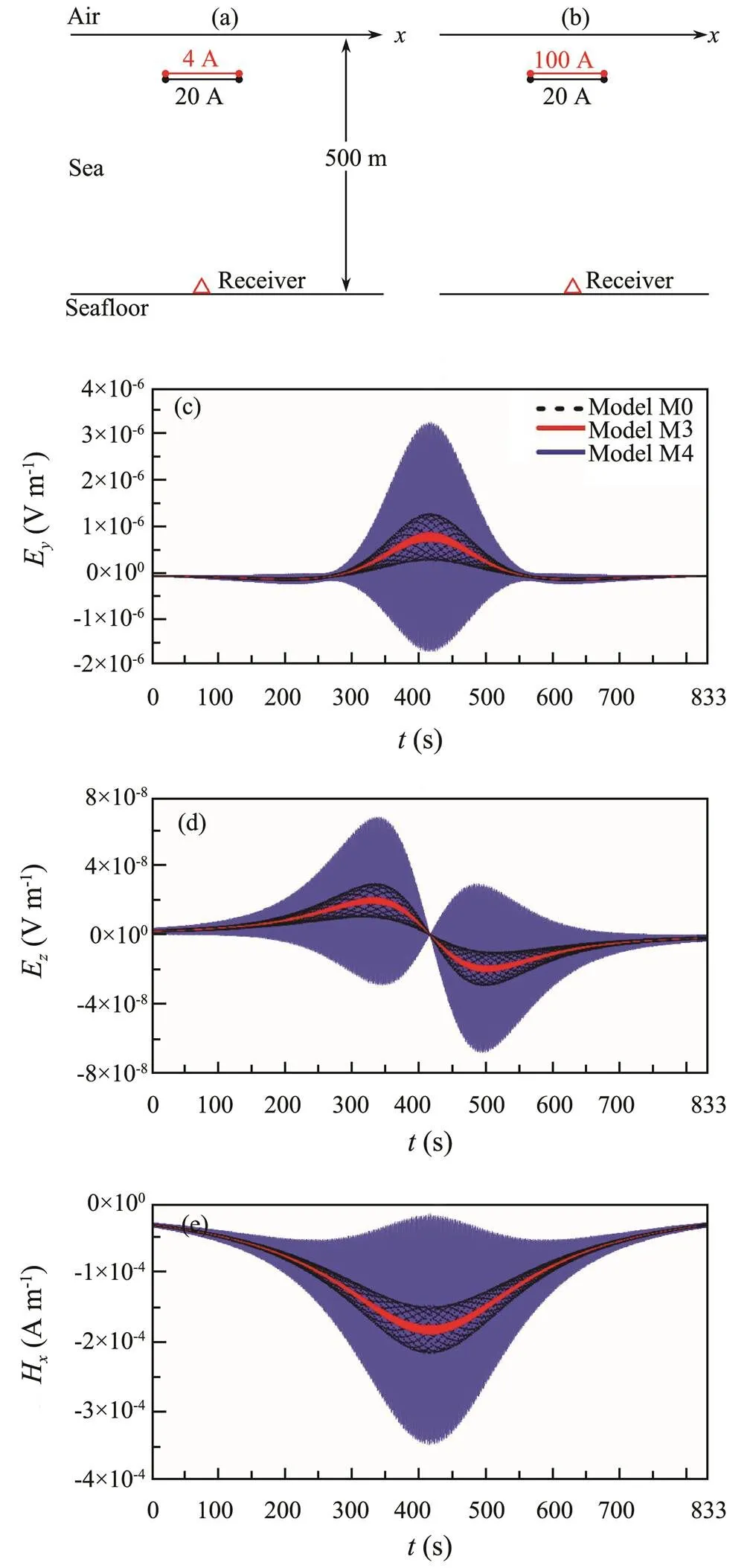
Fig.6 Schematic diagrams of (a) model M3 and (b) model M4 and the simulated results of (c) Ey, (d) Ez, and (e) Hx to illustrate the effects of alternating current intensity on the EMFMS.

Fig.7 Schematic diagrams of (a) model M5 and (b) model M6 and the simulated results of (c) Ey, (d) Ez, and (e) Hx to illustrate the effects of the source position on the EM- FMS.

By comparing Figs.7 and 8, one can find that when the seawater depth is much larger than the length of the current source, the source position has very little influence on the EMFMS, and vice versa. There are two reasons for this. One is that the shaft-rate field is of the same order in magnitude as the static field in shallow water. The other is the offsets of symmetric centers between the shaft-rate field and the static field are much larger in shallow water than in deep water.

3.3 Combined Effect of HED and VED Sources

In order to investigate the combined effect of HED and VED sources on EMFMS, we build the model M9 and M10. In model M9, there is a HED source, and both the alternating and static horizontal dipole sources are located at the same position and their positive and negative electrodes are at (−25, 0, 15) and (+25, 0, 15), respectively, as shown in Fig.9a. In model M10, the dipole source is tilted at an angle of 30˚ relative to the-axis and its center is at (, 0, 15), as shown in Fig.9b. The simulated EM- FMS of both models are shown in Figs.9c–9e.

From Figs.9c–9e, one can see that for the tilted dipole source (model M10), the electric fields are no longer symmetrical with respect to the axis of=416.5s. The electrical field amplitude on the left side becomes smaller and that on the right side becomes larger, and the amplitude of the magnetic field is smaller than that due to the horizontal dipole source (model M9). It is obvious that these features are resulting from the combined effect of the HED and VED sources.

Fig.8 Schematic diagrams of (a) model M7 and (b) model M8 and the simulated results of (c) Ey, (d) Ez, and (e) Hxto illustrate the effect of the source position on the EMFMS in shallow water.

Fig.9 Schematic diagrams of (a) model M9 and (b) model M10 and the simulated results of (c) Ey, (d) Ez, and (e) Hxto illustrate the combined effect of HED and VED sources.

4 Measured Data

We conducted an EMFMS test in the South Yellow Sea. An ocean bottom EM receiver (OBEM) was positioned on the seabed and recorded three electric field components and two horizontal components of the magnetic field. The sampling rate is 500Hz, and the water depth is 37m.

The research vessel ‘’ traveled across over the OBEM. The recorded data are processed. The shaft-rate of the vessel is about 3.667Hz.

Figs.10a and 10b show the measuredEand Hfields during a period of 216s, respectively. The measured fields are divided into the shaft-rate field and static field by using the sliding window technique (Figs.10c and 10d).

From Figs.10c and 10d, one can see the following features.

1) The anomaly of the shaft-rate magnetic field is greater than the shaft-rate electric field (in SI unit).

2) TheEcomponent and theHcomponent of the sta- tic field in Figs.10c and 10d are very similar to the static fields in Figs.4d and 4e.

3) The amplitude of static magnetic field is much larger than that of the shaft-rate magnetic field.

From the time-frequency spectrograms (Figs.10e and 10f), one can see the following features:

1) The static electric field is dominated at a frequency very close to 0Hz and the shaft-rate field is very clear at the fundamental frequency of 3.67Hz and its harmonics.

2) The amplitude of the static magnetic field is much larger than the shaft-rate magnetic field, which is generated by the metal material of the vessel.

Fig.10 Time series of (a) Ey and (b) Hx for measured EMFMS, time series of (c) Ey and (d) Hx for shaft-rate EM field and static field and spectrogram of (e) Ey and (f) Hx for EMFMS.

5 Conclusions

In this paper, we present a simulation method of electric and magnetic fields of a moving ship (EMFMS), which consisted of both the shaft-rate field generated by alterna- ting electric currents and the static field excited by static electric current. Then we investigated the effects of the current intensity and the source positions on the EMFMS. The numerical simulation and real measured data show that the seafloor, the shaft-rate field and the static field all have great impacts on EMFMS, so none of them could be neglected for EMFMS study.

Acknowledgements

This study is supported by the Fundamental Research Funds for the Central Universities (No. 201861020) and the Wenhai Program of Qingdao National Laboratory for Marine Science and Technology (QNLM) (No. 2017WH ZZB0201). We thank Drs. Ying Liu, Yunju Wu, Jie Lu, and Baoqiang Zhang for helpful suggestions on formula derivation of shaft-rate EM fields and data processing. We also thank two anonymous reviewers for valuable comments on our manuscript.

Bao, Z., Gong, S., Sun, J., and Li, J., 2011. Localization of a horizontal electric dipole source embedded in deep sea by using two vector-sensors., 23 (3): 53-57, DOI: 10.3969/j.issn.1009-3486.2011. 03.012 (in Chinese with English abstract).

Cheng, R., Jiang, R., and Gong, S., 2016. Calculation method of vessels’ shaft rate electric field equivalent source magnitude., 38 (2): 138-143, DOI: 10.11887/j.cn.201602023 (in Chinese with Eng- lish abstract).

Holmes, J., 2006.. Morgan & Claypool Publishers, London, 78pp.

Holtham, P., Jeffrey, I., Brooking, B., and Richards, T., 1999. Electromagnetic signature modeling and reduction.. London, UK, 97-100.

Jeffrey, I., and Brooking, B., 1999. A survey of new electromagnetic stealth technologies.. Biloxi, Mississippi, 1-7.

Li, D., Chen, C., Liu, H., and Yang, S., 2012. Green function method for extrapolating of ship’s underwater static electric field., 24 (3): 1-6, DOI: 10.3969/j.issn.1009-3486.2012.03.001 (in Chinese with English abstract).

Li, Y., and Li, G., 2016. Electromagnetic field expressions in the wavenumber domain from both the horizontal and vertical electric dipoles., 13 (4): 505-515, DOI: 10.1088/1742-2132/13/4/505.

Liu, S., Xiao, C., and Gong, S., 2004. Electromagnetic field of DC electric dipole in two-layer model., 28 (5): 641-644, DOI: 10.3963/j.issn.2095-3844.2004.05. 004 (in Chinese with English abstract).

Liu, Y., 2009. The measurement method of ship’s electric field. Master thesis. Harbin Engineering University (in Chinese with English abstract).

Lu, X., Gong, S., Zhou, J., and Liu, S., 2005. Quasi-near field localization of a time-harmonic HED in sea water., 29 (3): 331-334, DOI: 10.3963/j.issn.2095-3844. 2005.03.001 (in Chinese with English abstract).

Lu, X., Gong, S., Zhou, J., and Sun, M., 2004. Analytical expressions of the electromagnetic fields produced by an ELF time-harmonic HED embedded in the sea., 19 (3): 290-295, DOI: 10.13443/j.cjors.2004. 03.008 (in Chinese with English abstract).

Nain, H., Isa, M. C., Mohd, M., Yusoff, N. H. N., Yati, M. S. D., and Nor, I. M., 2013. Management of naval vessel’s electromagnetic signatures: A review of sources and countermeasures., 6 (2): 93-110.

Ni, H., Sun, M., and Gong, S., 2006. Calculation of the electromagnetic fields generated by horizontal current element in semi-infinite space of seawater., 20 (1): 63-65, DOI: 10.3969/j.issn. 1672-1497.2006.01.016 (in Chinese with English abstract).

Press, W. H., Flannery, B. P., Teukolsky, S. A., and Vetterling, W. T., 1992.. Press Syndicate of the University of Cambridge, New York, 1574pp.

Sun, M., Gong, S., Zhou, J., and Lu, X., 2003. Calculation of the electromagnetic fields generated by DC horizontal current element in semi-infinite space of seawater.. Istanbul, Turkey, 734-736.

Zhang, J., and Wang, X., 2016. Arithetic research about electric- field intensity of horizontal-harmonic current in the deep sea., 38 (1): 90-93, DOI: 10.3404/j. issn.1672-7649.2016.1.019 (in Chinese with English abstract).

Zolotarevskii, Y. M., Bulygin, F. V., Ponomarev, A. N., Narchev,V. A., and Berezina, L. V., 2005. Methods of measuring the low- frequency electric and magnetic fields of ships., 48 (11): 1140-1144, DOI: 10.1007/s11018-006- 0035-6.

. E-mail: yuguo@ouc.edu.cn

September 18, 2019;

February 26, 2020;

April 18, 2020

(Edited by Chen Wenwen)