AN Zhenfang, ZHANG Jin, *, and XING Lei

Inversion of Oceanic Parameters Represented by CTD Utilizing Seismic Multi-Attributes Based on Convolutional Neural Network

AN Zhenfang1), 2), ZHANG Jin1), 2), *, and XING Lei1), 2)

1),,,266100,2),,266071,

In Recent years, seismic data have been widely used in seismic oceanography for the inversion of oceanic parameters represented by conductivity temperature depth (CTD). Using this technique, researchers can identify the water structure with high horizontal resolution, which compensates for the deficiencies of CTD data. However, conventional inversion methods are model- driven, such as constrained sparse spike inversion (CSSI) and full waveform inversion (FWI), and typically require prior deterministic mapping operators. In this paper, we propose a novel inversion method based on a convolutional neural network (CNN), which is purely data-driven. To solve the problem of multiple solutions, we use stepwise regression to select the optimal attributes and their combination and take two-dimensional images of the selected attributes as input data. To prevent vanishing gradients, we use the rectified linear unit (ReLU) function as the activation function of the hidden layer. Moreover, the Adam and mini-batch algorithms are combined to improve stability and efficiency. The inversion results of field data indicate that the proposed method is a robust tool for accurately predicting oceanic parameters.

oceanic parameter inversion; seismic multi-attributes; convolutional neural network

1 Introduction

Oceanic parameters, including temperature, salinity, den- sity, and velocity can be obtained directly by conductivity temperature depth (CTD) instruments or indirectly by in- version utilizing seismic data. Although the vertical resolution of CTD data is higher than that of seismic data, its horizontal resolution is far lower. Joint CTD-seismic inversion combines the advantages of both to obtain oceanic parameters with high resolution.

However, traditional inversion methods, such as constrained sparse spike inversion (CSSI) and full waveform inversion (FWI), typically assume the existence of prior deterministic mapping operators between the geophysical responses and the geophysical parameters, such as a convolution operator and a wave equation operator. For some oceanic parameters, however, such as temperature and salinity, it is difficult to establish their mapping relationships and seismic responses by mathematical modeling.

A recent trend in many scientific fields has been to solve inverse problems using data-driven methods and a revived use of deep neural networks (DNNs). According to the universal approximation theorem (Hornik., 1990), a DNN can theoretically approximate any conti- nuous function when there are enough neurons in the hidden layer. Machine learning based on a DNN is usually referred to as deep learning. The convolutional neural network (CNN) is a DNN that has two special characteristics: local connection and shared weights, which improves computational efficiency by reducing the number of weights. Due to the significant advances in image pro- cessing and speech recognition, CNNs have attracted wide- spread attention and have been successfully applied in the fields of agriculture (Kamilaris and Prenafeta-Boldú, 2018; Qiu., 2018; Teimouri., 2018), medicine (Liu., 2017; Acharya., 2018; Wachinger., 2018), and transportation (Li and Hu, 2018; Li., 2018; Wang., 2018a).

Here, we introduce CNNs into marine geophysics to solve the inverse problem described above. Using deep learning, a CNN can automatically search and gradually approximate inverse mapping operators from the seismic responses to oceanic parameters, thus eliminating the need for prior deterministic mapping operators. In other words, CNN is purely data-driven.

In solid geophysics, CNNs are mainly applied to classification problems, such as fault interpretation (Guo., 2018; Ma., 2018; Wu., 2018a), first-break picking (Duan., 2018; Hollander., 2018; Yuan., 2018), seismic facies identification (Dramsch and Lüthje, 2018; Zhao, 2018), and seismic trace editing (Shen., 2018). Inversion belongs to the category of regression techniques. Generally, seismic inversion based on a CNN takes seismic records as input data and stratigraphic parameters as output data. In one study, generated normal- incidence synthetic seismograms served as input data, and the acoustic impedance served as output data (Das., 2018). In another study, synthetic two-dimensional multi- shot seismic waves were encoded into a feature vector, then the feature vector was decoded into a two-dimen- sional velocity model (Wu., 2018b). In a third study, a modified fully convolutional network was tuned to map pre-stacked multi-shot seismic traces to velocity models (Wang., 2018b).

The inversion methods mentioned above use one- or two-dimensional seismic records as input data and the corresponding subsurface models as output data. To obtain a large number of samples, many subsurface models are built to generate synthetic seismic records. These methods have made some progress, but continue to have a number of disadvantages. First, they require prior deterministic forward operators to synthesize the seismic records. Second, accurate inversion results cannot be obtained based on a small number of samples. Third, the problem of multiple solutions becomes more prominent as only seismic records are used as input data.

The samples for our study were obtained from actual data, including both CTD and seismic data acquired from the East China Sea. We took the CTD curves as output data and the seismic traces near the CTDs as input data. Given the fact that if only seismic records are used as input data, the problem of multiple solutions inevitably arises, to re- duce the multiplicity of solutions, we used stepwise regre- ssion to select only the optimal attributes and their combination and took the two-dimensional images of the selected attributes as input data. Because of the frequency difference between the CTD and seismic data, we assumed that one sampling point on the CTD curve corresponded to multiple adjacent sampling points on the seismic trace near the CTD.

2 Theory of Convolutional Neural Networks

CNNs (Venkatesan and Li, 2018) consist of an input layer, hidden layers, and an output layer. The hidden layers between the input and output layers generally consist of convolution layers, pooling layers, and a fully connectedlayer. Each hidden layer incorporates several feature maps, and each feature map contains one or more neurons. Fig.1 shows the architecture of the CNN designed for this study, the model parameters of which are listed in Table 1.

The CNN workflow can be divided into forward and backward propagation. Model output can be obtained afteran original image is successively processed by convolution, pooling, and its weighted sums during forward propagation. Then, the error between the model output and the de- sired output propagates backward from the output layer to the first hidden layer. Meanwhile, the convolution kernels, weights, and biases are updated during backward propagation. These updates will continue until the error tolerance value is reached.

Fig.1 Architecture of the convolutional neural network, wherein the squares represent maps of neurons. The number on the left of @ denotes the number of maps, and the two numbers on the right of @ denote the number of rows and columns in the map, respectively.

Table 1 Model parameters of the convolutional neural network

2.1 Forward Propagation

For this process, let the current layer be layer, and the layer in front of the current layer be layer−1.

The convolution layer can be obtained as follows:

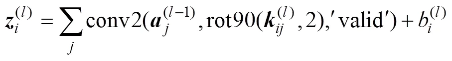
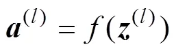
where(l−1)represents the original image of the input layer or the output of the pooling layer;(l)andb(l)are the convolution kernel and the bias of the convolution layer, respectively;(l)and(l)are the input and output of the convolution layer, respectively; rot90(·) performs the 180-degree counterclockwise rotation of(l); conv2(·) performs the two-dimensional convolution of(l−1)and(l), wherevalidreturns only those parts of the convolution that are computed without zero-padded edges; and(·) denotes the activation function.

The pooling layer can be obtained by the following:

where(l−1)represents the output of the first convolution layer;(l)and(l)are the input and output of the pooling layer, respectively; and down(·) performs the down-sampling operation of(l−1).

The fully connected layer and the output layer can be obtained as follows:

where(l−1)represents the output of the second convolution layer or the fully connected layer;(l)and(l)are the weight and bias of the fully connected layer or the output layer, respectively;(l)and(l)are the input and output of the fully connected layer or the output layer, respectively; and the symbol * denotes multiplication between the two matrices. In the setting=(L),is the total number of layers.

To prevent vanishing gradients, we use a rectified linear unit (ReLU) function (Nair and Hinton, 2010) as the activation function of the hidden layer. Because the desired output is normalized during data preprocessing, we use the sigmoid function as the activation function of the output layer.

2.2 Backward Propagation

Learning rules are driven by the cost function, which is defined as follows:

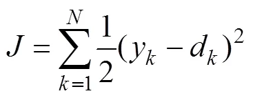
whereyanddare the model output and the desired output, respectively,is the number of data points, andis the cost function.

According to the gradient descent method, the convolution kernels, weights, and biases are updated as follows:

whereis the learning rate anddenotes the convolution kernel, the weight, or the bias.

The partial derivatives ofwith respect to(l)and(l)of the output layer and the fully connected layer can be calculated as follows:

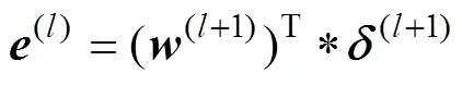
where the superscript T represents the transpose of(l−1)and(l)denotes the delta of the output layer or the fully connected layer. The delta is defined as the element- by-element multiplication of the error and the derivative of the weighted sum:

where the symbol ·* denotes element-by-element multiplication and(l)is the error of the output layer:

or the error of the fully connected layer:

The partial derivatives ofwith respect to(l)andb(l)of the convolution layer can be calculated as follows:

where sum(·) performs summation of the elements of(l). The delta of the convolution layer can be obtained using Eq. (11). The error of the second convolution layer can be obtained using Eq. (13). Because down-sampling is performed from the first convolution layer to the pooling layer during forward propagation, up-sampling should be performed from the pooling layer to the first convolution layer during backward propagation. The error of the first convolution layer can be obtained by the following:

, (16)

where up(·) performs the up-sampling operation of(l+1).

The error of the pooling layer can be calculated as follows:

wherefullreturns the full two-dimensional convolution.

3 Methodology Used to Perform Inversion

The CTD data and the seismic data near the CTD are different responses at the same sea-water location, so they have an inherent relationship that can be approximated by the CNN. First, the CTD curves are taken as the desired output data and the seismic traces near the CTDs are taken as the input data. The CNN automatically approximates the inverse mapping operator from the input data to the desired output data. Then, the seismic traces obtained far away from the CTDs are input into the trained network model that serves as the inverse mapping operator. Finally, the inversion results are output from the network model.

3.1 Input and Output of Convolutional Neural Network

The CTD curves and the seismic traces near the CTDs are taken as the desired output data and the input data, respectively. If only seismic records are taken as input data, the problem of multiple solutions inevitably arises. To solve this problem, stepwise regression is performed to select the optimal attributes and their combination, including the instantaneous frequency, instantaneous amplitude, instantaneous phase, average frequency, dominant frequency, apparent polarity, and the derivative, integral, coordinate, and time attributes. Then, we take the two-dimensional images of the selected attributes as input data instead of the one-dimensional seismic records. The selected attributes are the derivative, time and-coor- dinate, which are located in the left-hand, middle, and right-hand columns of the images, respectively.

Because the frequency of CTD data differs from that of seismic data, their sampling points do not have a one- to-one correspondence, but one-to-many. We assume that one sampling point in the CTD data corresponds to five adjacent sampling points near the CTD in the seismic data. As shown in Fig.2, we took images with 5×3 pixels as input data and the corresponding target point as the desired output data.

3.2 Optimization of Training for Network Model

We divided the samples into training and validation datasets and used cross validation to determine whether the network model was overfitting the data. The root-mean- square error (RMSE) between the model and desired out- puts is defined as follows:

where e is the RMSE, yk and dk are the model and desired outputs, respectively, and N is the number of data points. If the RMSE of the validation dataset is consistently too large, this indicates that the network model is overfitting.

The training dataset was evenly divided into several groups, and the convolution kernels, weights, and biases were not updated until all the samples in one group had been trained. This optimization method, known as the mini- batch algorithm, has the high efficiency of the stochastic gradient descent (SGD) algorithm and the stability of the batch algorithm. If the training dataset is kept as just one group, the mini-batch algorithm becomes a batch algorithm. If each group has only one sample, the mini-batch algorithm becomes an SGD algorithm. The increments of the convolution kernels, weights, and biases are calcula- ted by the SGD and batch algorithms shown in Eqs. (19) and (20), respectively:

whereis the convolution kernel, the weight, or the bias, and Δis the increment of convolution kernel, weight, or bias.

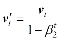
With the mini-batch algorithm, we combined another op-timization method, known as Adam (Kingma and Ba, 2015), the name of which is derived from adaptive moment esti- mation. Adam combines the advantages of the AdaGrad and RMSProp algorithms, and works well with sparse gradients as well as in non-stationary settings. In the Adam algorithm, convolution kernels, weights, and biases are updated as follows:

whereis the convolution kernel, the weight, or the bias; the subscriptis the timestep, making=+1, with0=0 as the initialized timestep;is the learning rate;is a very small value; and′ and′ are the bias-corrected first moment estimate and the bias-corrected second raw- moment estimate, respectively:

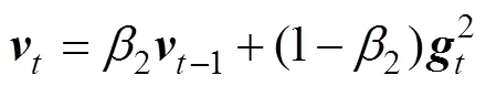
where1and2are the exponential decay rates for the respective moment estimates, andandare the biased first moment estimate and the biased second raw-moment estimate, respectively:

where0=0 and0=0 are the initialized first moment vector and the initialized second raw-moment vector, respectively, andis the gradient with respect to the stochastic objective function, namely the vector of the partial derivatives of() with respect toevaluated at timestep:

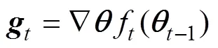
where() denotes the stochastic objective function with parameter. Good default settings for the tested machine learning problems are=0.001,1=0.9,2=0.999, and=10−8. In this study, however,=0.0001, because the mo- del output will fluctuate around the true solution when=0.001. All operations on vectors are element-wise.

4 Field Data

A post-stack seismic profile (Fig.3) with 1000 traces was acquired from the East China Sea, and three CTDs were dropped near the seismic traces numbered 85, 471, and 854. It is difficult to distinguish vertical variations in the ocean water from Fig.3 due to its low vertical resolution, which shows only the strong reflection interface. Fig.4 shows the temperature, salinity, density, and velocity curves plotted using data from CTD-1, CTD-2, and CTD- 3, in which we can see that temperature and velocity decrease with depth, whereas salinity and density increase with depth.

Figs.5, 6, and 7 show the selected derivative, time, and-coordinate attributes obtained using stepwise regression. The derivative attribute is the nonlinear transformation of the seismic data, which records differences in amplitude values between adjacent sampling points. We know that the frequency of seismic data is much lower than that of the CTD data, but the frequency difference between them decreases significantly with the increased high-frequency component after derivative processing, which improves the correlation between the seismic and CTD data. Use of the coordinate attribute can reduce the multiplicity of solutions and improve generalizability. Because CTD data is converted from the depth domain to the time domain, time takes the place of the-coordinate.

CNNs tend to overfit data when the number of samples is small. To avoid overfitting, we obtained six virtual CTDs by linear interpolation between the three actual CTDs to supply the CNN with more samples. For testing, we used CTD-2 and the seismic attributes extracted from the seismic trace numbered 471, and used the other eight pairs of inputs and outputs for training.

4.1 Data Preprocessing

CTD and seismic data are in different domains, so we converted the CTD data to the time domain using the following depth-time conversion equation:

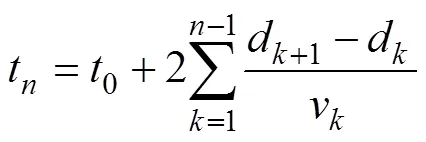
whereis the interval velocity,is the depth for each interval velocity,0is the two-way vertical time to1, andtis the two-way vertical time corresponding tod.

Due to the differences in the dimensions and units of the seismic attributes and the oceanic parameters, it is dif- ficult for the CNN to converge if these attributes and parameters are directly used for training. Therefore, we no- malized the seismic attributes and oceanic parameters using Eqs. (28) and (29), respectively:

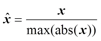
Fig.4 Oceanic parameters measured by CTD-1 ((a) and (d)), CTD-2 ((b) and (e)), and CTD-3 ((c) and (f)), which are located near the seismic traces numbered 85, 471, and 854, respectively. The blue, green, red, and cyan lines denote the temperature, salinity, density, and velocity curves, respectively.

Fig.5 Derivative attribute profile.

Fig.6 Time attribute profile.

Fig.7 x-coordinate attribute profile.

where abs(·) represents the absolute value of the elements of, and max(·) and min(·) are the largest and smallest elements in, respectively.

4.2 Inversion of Oceanic Parameters Represented by CTD

Four network models were established for inverting tem- perature, salinity, density, and velocity. After 10000 epo- chs, the four network models ended training as the error tolerance had been reached, as shown in Fig.8.

A series of images containing 5×3 pixels were then ge- nerated from the three attribute profiles shown in Figs.5, 6, and 7. These images were then input into the four trained network models in turn. Finally, the predicted temperature, salinity, density, and velocity profiles were quickly output, as shown in Figs.9–12, respectively.

Figs.3 and 9–12 show different responses to the same sea water, with Fig.3 reflecting the variation of impedance and Figs.9–12 reflecting the respective variations of temperature, salinity, density, and velocity. The vertical resolutions of Figs.9–12 as compared with that of Fig.3 have improved.

Fig.8 Error variation with epoch. The blue, green, red, and cyan lines represent the error curves of temperature, salinity, density, and velocity, respectively.

Since the desired outputs were normalized in data preprocessing, the model outputs were then post-processed using the following inverse transformation equation:

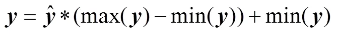
Fig.10 Salinity profile predicted by convolutional neural network.

Fig.11 Density profile predicted by convolutional neural network.

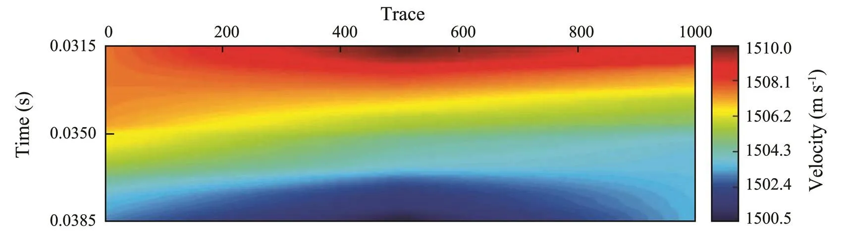
Fig.12 Velocity profile predicted by convolutional neural network.

The accuracy of the inversion results can be determined by comparing the model outputs with the desired outputs in the location of CTD-2. Fig.13 shows fold plots of the model and desired outputs, in which we can see that the predicted and actual oceanic parameters exactly match, and the Pearson correlation coefficients of the four oceanic parameters exceed 90%. Therefore, we can conclude that the proposed method is confirmed to have generalizability for accurately predicting temperature, salinity, density, and velocity.

Fig.13 Fold plots of the predicted and actual oceanic parameters in the location of CTD-2. The blue solid and red dotted lines denote the desired and model outputs, respectively.

5 Conclusions

It is difficult for the traditional seismic inversion me- thod to establish mapping relationships between oceanic parameters and seismic responses by mathematical modeling. In this paper, we presented a CTD-seismic joint in- version method based on a CNN, which is purely data- driven. Using deep learning, the CNN can automatically approximate the inverse mapping operator from input data to the desired output data. To reduce the multiplicity of solutions, we utilized stepwise regression to select the best attributes and their combination and took the two- dimensional images of the selected attributes as input data. The derivative attribute was shown to improve the correlation between the seismic and CTD data, and the coordinate attribute to reduce the multiplicity of solutions and improve generalizability. The inversion results of our field data proved that the proposed method can accurately predict oceanic parameters.

Joint CTD-seismic inversion based on CNN is data- driven, which gives it bright prospects for the future, although a number of problems remain to be solved. Among them the most prominent is the multiplicity of solutions. To reduce the multiplicity of solutions, existing appro- aches basically involve increasing the number of samples. However, the resulting trained network model is still only applicable to local areas. This is an urgent problem that must be addressed to further reduce the multiplicity of so- lutions and improve generalizability.

Acknowledgements

This research is jointly funded by the National Key Research and Development Program of China (No. 2017 YFC0307401), the National Natural Science Foundation of China (No. 41230318), the Fundamental Research Funds for the Central Universities (No. 201964017), and the National Science and Technology Major Project of China (No. 2016ZX05024-001-002).

Acharya, U. R., Fujita, H., Oh, S. L., Raghavendra, U., Tan, J. H., Adam, M., Gertych, A., and Hagiwara, Y., 2018. Automated identification of shockable and non-shockable life- threatening ventricular arrhythmias using convolutional neural network., 79: 952- 959.

Das, V., Pollack, A., Wollner, U., and Mukerji, T., 2018. Convolutional neural network for seismic impedance inversion.. Anaheim, 2071-2075.

Dramsch, J. S., and Lüthje, M., 2018. Deep learning seismic facies on state-of-the-art CNN architectures.. Anaheim, 2036-2040.

Duan, X. D., Zhang, J., Liu, Z. Y., Liu, S., Chen, Z. B., and Li, W. P., 2018. Integrating seismic first-break picking methods with a machine learning approach.. Anaheim, 2186-2190.

Guo, B. W., Liu, L., and Luo, Y., 2018. A new method for automatic seismic fault detection using convolutional neural network.. Anaheim, 1951-1955.

Hollander, Y., Merouane, A., and Yilmaz, O., 2018. Using a deep convolutional neural network to enhance the accuracy of first break picking.. Anaheim, 4628-4632.

Hornik, K., Stinchcombe, M., and White, H., 1990. Universal approximation of an unknown mapping and its derivatives using multilayer feedforward networks., 3 (5): 551-560.

Kamilaris, A., and Prenafeta-Boldú, F. X., 2018. Deep learning in agriculture: A survey., 147: 70-90.

Kingma, D. P., and Ba, J. L., 2015. Adam: A method for stochastic optimization.(). San Diego, 1-15.

Li, B., and Hu, X., 2018. Effective vehicle logo recognition in real-world application using mapreduce based convolutional neural networks with a pre-training strategy., 34 (3): 1985-1994.

Li, Y., Huang, Y., and Zhang, M., 2018. Short-term load forecasting for electric vehicle charging station based on niche immunity lion algorithm and convolutional neural network., 11 (5): 1253.

Liu, F., Zhou, Z., Jang, H., Samsonov, A., Zhao, G., and Kijowski, R., 2017. Deep convolutional neural network and 3D deformable approach for tissue segmentation in musculoske-letal magnetic resonance imaging., 79 (4): 2379-2391.

Ma, Y., Ji, X., BenHassan, N. M., and Luo, Y., 2018. A deep learning method for automatic fault detection.. Anaheim, 1941-1945.

Nair, V., and Hinton, G. E., 2010. Rectified linear units improve restricted Boltzmann machines.(). Omnipress, 807-814.

Qiu, Z., Chen, J., Zhao, Y., Zhu, S., He, Y., and Zhang, C., 2018. Variety identification of single rice seed using hyperspectral imaging combined with convolutional neural network., 8 (2): 212.

Shen, Y., Sun, M. Y., Zhang, J., Liu, S., Chen, Z. B., and Li, W. P., 2018. Seismic trace editing by applying machine learning.. Anaheim, 2256- 2260.

Teimouri, N., Dyrmann, M., Nielsen, P., Mathiassen, S., Somer- ville, G., and Jørgensen, R., 2018. Weed growth stage estimator using deep convolutional neural networks., 18 (5): 1580.

Venkatesan, R., and Li, B. X., 2018.:. CRC Press, Boca Raton, 1-183.

Wachinger, C., Reuter, M., and Klein, T., 2018. DeepNAT: Deep convolutional neural network for segmenting neuroanatomy., 170: 434-445.

Wang, Q., Gao, J., and Yuan, Y., 2018a. A joint convolutional neural networks and context transfer for street scenes labeling., 19 (5): 1457-1470.

Wang, W. L., Yang, F. S., and Ma, J. W., 2018b. Velocity model building with a modified fully convolutional network.. Anaheim, 2086-2090.

Wu, X. M., Shi, Y. Z., Fomel, S., and Liang, L. M., 2018a. Con- volutional neural networks for fault interpretation in seismic images.. Ana- heim, 1946-1950.

Wu, Y., Lin, Y. Z., and Zhou, Z., 2018b. InversionNet: Accurate and efficient seismic waveform inversion with convolutional neural networks.. Anaheim, 2096-2100.

Yuan, S. Y., Liu, J. W., Wang, S. X., Wang, T. Y., and Shi, P. D., 2018. Seismic waveform classification and first-break picking using convolution neural networks., 15 (2): 272-276.

Zhao, T., 2018. Seismic facies classification using different deep convolutional neural networks.. Anaheim, 2046-2050.

. E-mail: zhjmeteor@163.com

January 30, 2019;

May 10, 2019;

May 6, 2020

(Edited by Chen Wenwen)