周海蓉，田 雨，饶长辉*

稀疏先验型的大气湍流退化图像盲复原

周海蓉1,2,3，田 雨1,2，饶长辉1,2*

1中国科学院自适应光学重点实验室，四川 成都 610209；2中国科学院光电技术研究所，四川 成都 610209；3中国科学院大学，北京 100049

图像盲复原是仅从降质图像就恢复出模糊核和真实锐利图像的方法，由于其病态性，通常需要加入图像先验知识约束解的范围。针对传统的图像梯度2和1范数先验不能真实刻画自然图像梯度分布的特点，本文将图像梯度稀疏先验应用于单帧大气湍流退化图像盲复原中。先估计模糊核再进行非盲复原，利用分裂Bregman算法求解相应的非凸代价函数。仿真实验表明，与总变分先验(1范数)相比，稀疏先验有利于模糊核的估计、产生锐利边缘和去除振铃等，降低了模糊核的估计误差从而提高了复原质量。最后对真实湍流退化图像进行了复原。

自适应光学；稀疏先验；盲解卷积；分裂Bregman

1 引 言

地基望远镜对太空目标(如卫星、恒星或太阳)观测时，受地球大气湍流影响，其成像分辨力远远低于衍射极限，通过自适应光学(adaptive optics, AO)系统能实时补偿湍流造成的波前畸变[1]，但由于系统自身存在误差如变形镜拟合误差、时间带宽误差和非等晕误差等，闭环校正后的图像仍然存在残差，需要进行事后处理以进一步提升图像质量。常用的事后处理方法有相位差法、斑点图像重建法和盲解卷积法。相位差法需要一套额外的成像装置，而斑点图像重建法则是利用上百帧短曝光的图像恢复出目标的相位和振幅信息[2]。与前两种方法相比，盲解卷积法仅需一帧或几帧降质图像即可实现重建，方法更显简单灵活。

盲复原算法在求解策略上可分为联合估计法和两阶段估计法，前者同时恢复出目标和模糊函数，后者先估计出模糊函数再进行非盲复原。Levin[3]表明传统的最大后验概率联合估计法MAP,k(maximum a posteriori, MAP)倾向于得到无模糊解导致复原失败，而MAP先估计出模糊核的两阶段方法会成功。无模糊解即复原图像为退化图像，复原模糊核为脉冲响应。但MAP,k方法在实际实验中取得成功[4]。为解决这个矛盾，Perrone[4]首先证明了Levin的正确观点，其次表明MAP,k成功原因在于归一化步骤是顺序进行的，因此MAP,k和MAP两种求解方法都是可行的，盲解卷积问题的关键还是在于先验的选择。

盲解卷积方法的困难之处在于方程存在无穷解，如真解和无模糊解(no-blur solution)都是问题的解。克服盲解卷积病态性的方法是通过加入先验来约束解的范围，从而避免不需要的解。传统的迭代盲解卷积算法(iterative blind deconvolution, IBD)使用正性约束和能量守恒约束进行交替求解，然而算法没有稳定收敛性保证[5]。Lane[6]将先验化为代价函数的一个正则化项，使用共轭梯度法进行联合求解，算法虽然克服了病态性问题但容易陷入局域解。Jefferies等[7]在Lane的基础上进一步优化，加入带宽有限约束和傅里叶模量约束。其后You和Kaveh[8]提出将图像梯度的1范数作为图像平滑约束，但由于1范数是各向同性的，在复原同时无法保留图像细节，Chan和Wong[9]在此基础上引入图像总变分(total variation, TV)约束，并设计了交替最小化的求解方案。与传统图像盲复原算法相比，当前算法都引入自然图像的统计信息作为先验，并广泛采用MAP两阶段估计法进行求解。Fergus[10]使用混合高斯模型对图像梯度进行建模，Krishnan[11]采用另一种图像先验1/2使得锐利图像的代价函数最小，并采用迭代再加权最小二乘(iterative reweighted least squares, IRLS)算法求解模糊核。Kotera等[12]采用图像梯度的稀疏范数l(0<<1)去除图像中的运动模糊。

真实的自然图像梯度[3]表现为稀疏的长拖尾分布。与传统的总变分先验[9]相比，稀疏范数l更能真实地刻画这种稀疏分布，常用于图像去运动模糊的盲复原领域[12]，本文将这种稀疏先验引入大气湍流降质图像的盲复原中。首先，稀疏先验将产生非凸的代价函数，本文采用分裂Bregman优化算法[13]和查表法[14]进行数值求解。其次，采用Krishnan[14]的稀疏先验方法复原出锐利图像，避免了Fergus等[10]出现的振铃现象。最后，分别对仿真的湍流退化图像和真实观测图像进行图像复原，验证了算法的有效性。

2 基于稀疏的盲解卷积复原算法

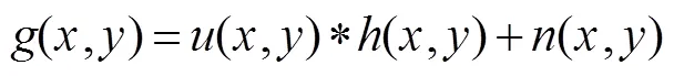
当前盲复原方法路线主要分为基于概率统计的贝叶斯法、正则化法以及变分贝叶斯估计，贝叶斯估计是假设图像、模糊核或噪声服从某种分布作为先验知识加入最大似然函数，先验即转化为代价函数中的正则化项，因此贝叶斯估计与正则化方法实际是等价的。用()表示真实图像，()为模糊核，()为噪声，()表示观测图像，“*”表示空域卷积，图像的线性退化过程可表示为

2.1 图像的统计模型

表1罗列了常用的图像先验模型，其中“Ñ”表示梯度算子。传统的盲复原算法采取的先验是基于图像的强度信息，如维纳滤波迭代盲解卷积假设图像强度服从高斯分布。其后学者采用图像的梯度作为先验，如You和Kaveh[6]使用梯度1范数(即Gaussian分布)，Chan[7]采用梯度的1范数(即Laplace分布)有利于保持边缘和细节。对自然图像的梯度进行统计时，其对数分布直方图如图1(a)所示，其统计分布为非高斯的长拖尾分布。若采用参数模型进行拟合，如图1(b)表明Gaussian先验和Laplace先验均不能近似这种分布，而稀疏先验(<1)更能近似真实图像梯度的长拖尾分布，这种先验有利于产生锐利的边缘、减少噪声并去除振铃现象[13]。

表1 常用的图像先验模型

2.2 算法框架

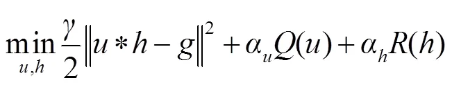
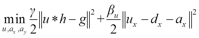
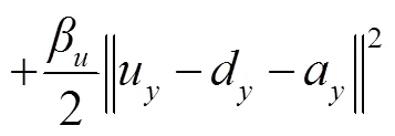
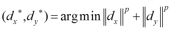
将稀疏先验和模糊核先验加入代价函数后的最小化目标函数为

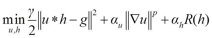
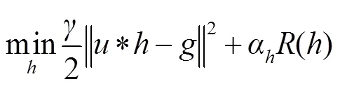
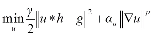
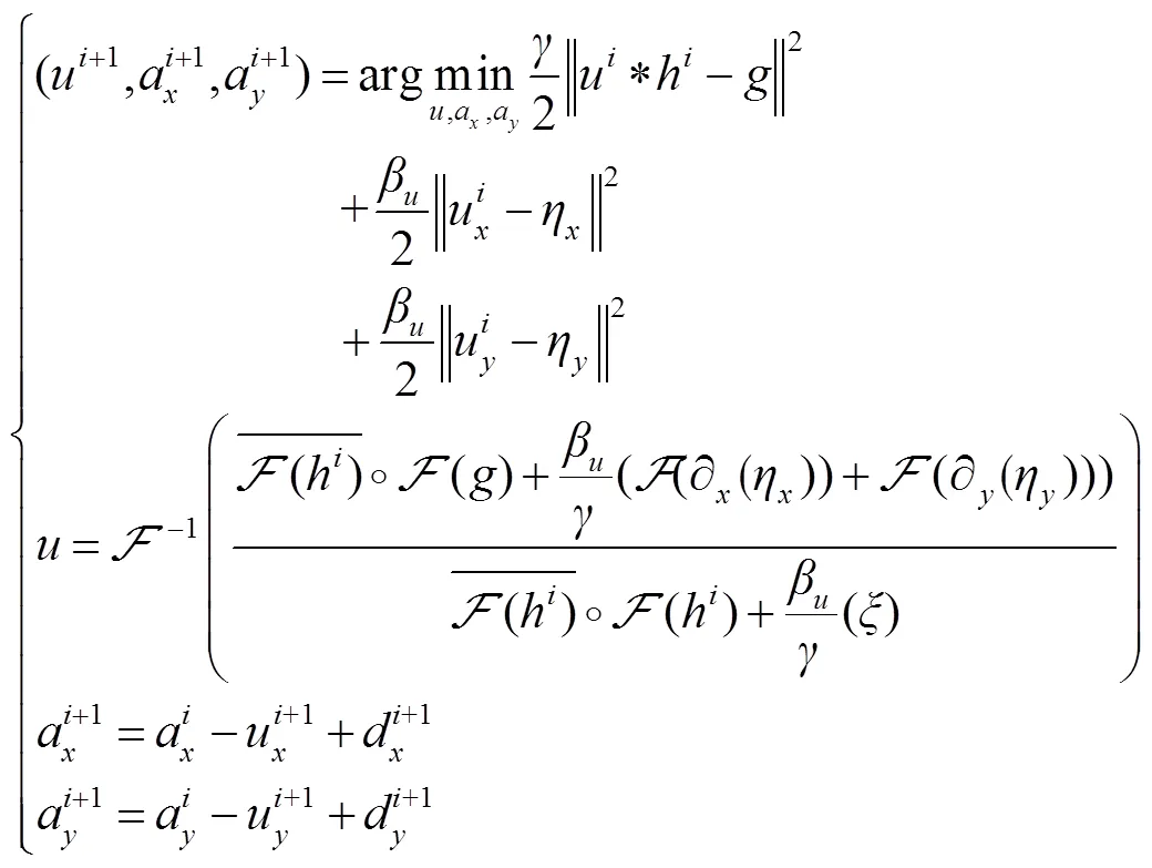
直接求解式(3)是困难的，Jefferies等[7]使用共轭梯度联合求解和，但Levin[3]表明这种联合求解策略容易陷入无模糊，采用先估计模糊核再非盲复原的两阶段方法会成功。本文采用交替最小化方案[9]可将式(3)转换为两个子问题交替求解。Chan[15]证明了交替最小化方案的收敛性，其中模糊核子问题和图像核子问题分别如下：

与总变分盲解卷积[9]类似，稀疏先验导致代价函数式(4)非凸，无法得到闭式解，需要进行迭代求得数值近似解。Levin[16]提出IRLS算法求解这种l范数最优化问题，但使用共轭梯度法需要迭代上百次。Goldstein[13]提出分裂Bregman算法求解总变分盲解卷积，Krishnan[14]提出查表法(look-up table, LUT)将分裂Bregman算法推广到求解含有l范数的非凸解卷积问题，算法速度比IRLS提高了几个数量级。本文采用分裂Bregman算法和查表法来求解上述两个子问题式(4)和式(5)。

2.2.1 模糊核子问题

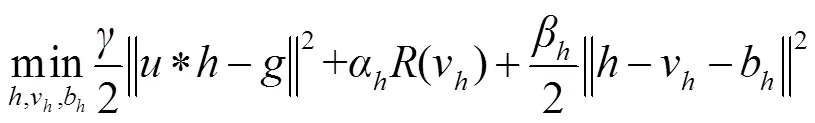
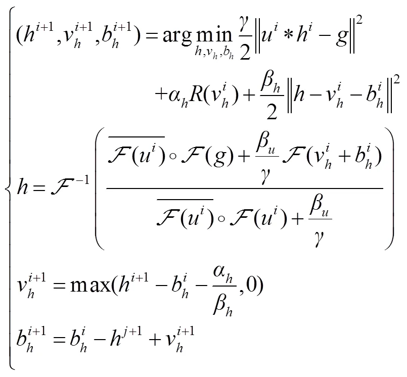
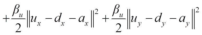
首先，由分裂Bregman算法思想，通过引入辅助变量v=h将式(4)化为一个有约束最小化问题，再引入Bregman变量b形成二次惩罚项进行迭代求解，为二次惩罚项的权重，最终的最小化目标函数为

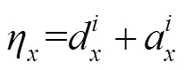
加入辅助变量后，可以推导出和v的频域闭式解，同时更新Bregman变量b，总的迭代求解过程如下：

图1 自然图像统计模型。(a) 真实自然图像的梯度分布；(b) 参数模型

Fig. 1 Natural images statistical model. (a) Real natural image gradient distribution; (b) Parametric model

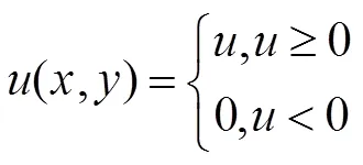
和归一化：

约束。

2.2.2 图像子问题

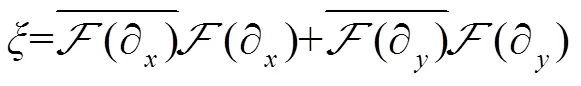
进行变量分离后，在频域推导出的闭式解，同时更新Bregman变量，求解过程如下：

其中：

2.2.3子问题

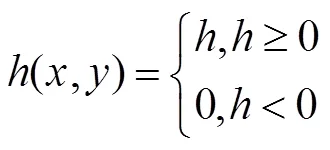
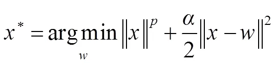
模糊核子问题中的变量v是存在闭式解的，可以用软阈值求解。而子问题是一个l范数非凸问题，其最小化方程为

等价于求解最小化问题：

当=1时，化为一个1正则化问题[13]，其解为

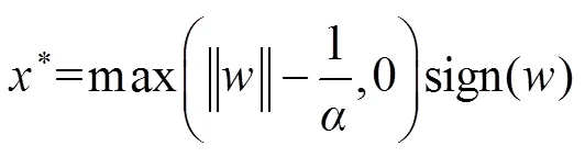
也写为

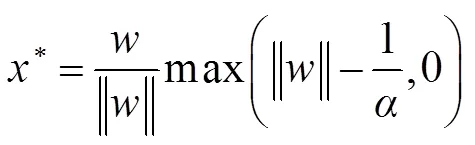
当0<<1时，采用Krishnan[11]查表法(lookup table, LUT)可得到近似解。

2.2.4 避免陷入局域解的策略

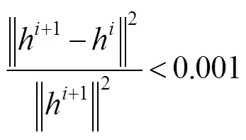
稀疏先验将导致卡通效应，在算法迭代时以1.5倍增大保真项的权重，即逐渐减小正则化的强度，有利于降低复原图像的分段平滑效应。此外，在每个子问题迭代时，迭代次数不宜过多，防止算法陷入局域解中[4]，设置算法的迭代停止条件：

3 实验结果与分析

3.1 大气湍流退化图像仿真实验

大气湍流是限制大型天文望远镜成像分辨率的主要原因，它造成的随机波前畸变可以用Zernike多项式表示。它的每一项都表示传统光学系统的基本像差，如离焦、像散和慧差等，这种方法得到的数值模拟效果比较符合Kolmogrov谱的湍流模型[17]。波前相位中的Zernike系数近似服从零均值的高斯分布(图2)。测试图像为OCNR5卫星(图3(a))，大小为256 pixels×256 pixels，降质图像为图3(b)，利用Zernike前65项多项式生成点扩散函数(point spread function, PSF)如图3(b)右下角所示。定义核估计的相对误差为

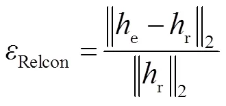
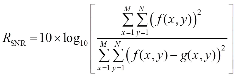
其中：hr为真实核，he为估计核。数值越小表示估计的核与真实核越接近。假设真实图像为f(x,y)，降质图像为g(x,y)，使用图像信噪比(signal to noise ratio, SNR)衡量复原图像的质量，数值越大说明复原质量越好，定义为

使用稀疏先验盲复原算法对降质图像进行复原，算法中的参数初始化为：，，，，。将复原结果与维纳滤波迭代盲复原和总变分盲复原进行对比，图3(c)~3(h)为三种算法的复原结果，图中右下角为对应的估计模糊核。从图3(c)可以看出，维纳滤波盲复原的PSF估计误差大，信噪比低，但仍恢复出目标的大尺度轮廓。总变分盲复原(图3(d))能保持更多的细节，估计的PSF结构和形状更接近真实的PSF，但仍存在残余模糊。图3(e)~(h)分别为使用p值为0.9、0.6、0.3和0.1的稀疏先验进行盲复原的结果，可以看出p的取值过大(p=0.9)时，出现了显著的振铃现象；而p的取值过小(p=0.1)时，核估计误差增大，细节和轮廓被噪声淹没；p的取值为0.6时，复原图像具有了丰富的细节和轮廓；当p的取值为0.3时，核估计误差最小，对应的复原图像信噪比值最高，复原质量最好。表2给出了不同算法的核估计误差和信噪比值。图4给出了三种算法的收敛情况，维纳滤波盲复原算法的核估计相对误差先是快速下降，但收敛缓慢，加入分裂Bregman算法优化后，总变分盲复原和稀疏先验盲复原算法都能稳定地收敛。

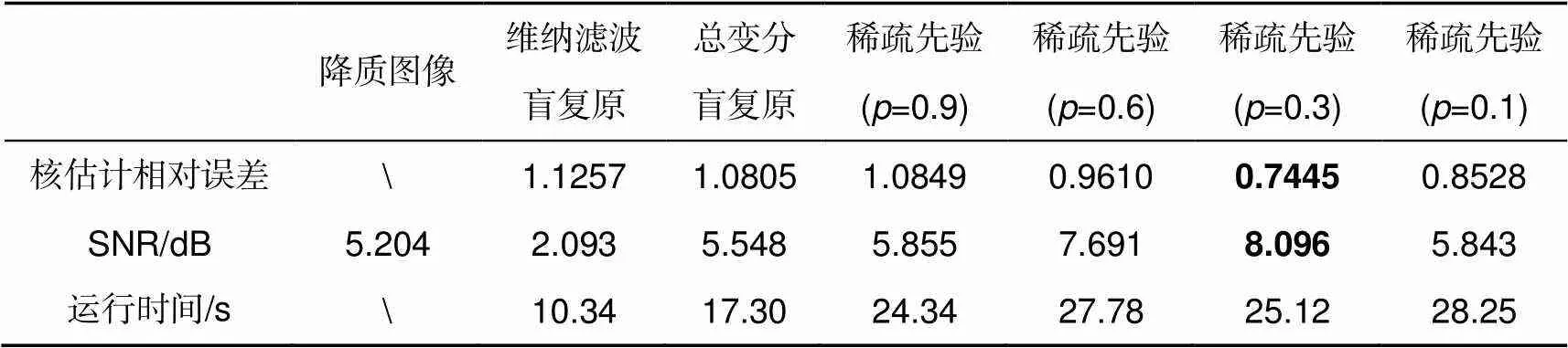
表2 不同算法的核估计误差和信噪比

表2还给出了不同算法的运行时间，维纳滤波盲复原算法直接在频域求得解析解，单个子问题不需要迭代，因此时间消耗少仅需10.34 s；在使用分裂Bregman算法进行数值计算后，总变分盲解卷积需要17.30 s；而稀疏先验盲解卷积算法由于图像子问题非凸需要查表，时间消耗为24.34 s(=0.9)、27.78 s(=0.6)、25.12 s(=0.3)和28.25 s(=0.1)。三种算法均是在Matlab2017Ra平台上运行，测试计算机系统为Window7旗舰版64位操作系统，处理器为AMD A10 PRO-7800B R7，12 Compute Cores 4C+8G @3.50 GHz，内存为8 G。

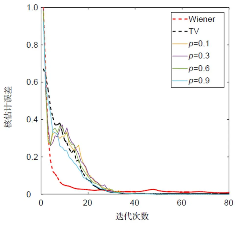
图4 算法收敛性比较

3.2 p值的选取原则

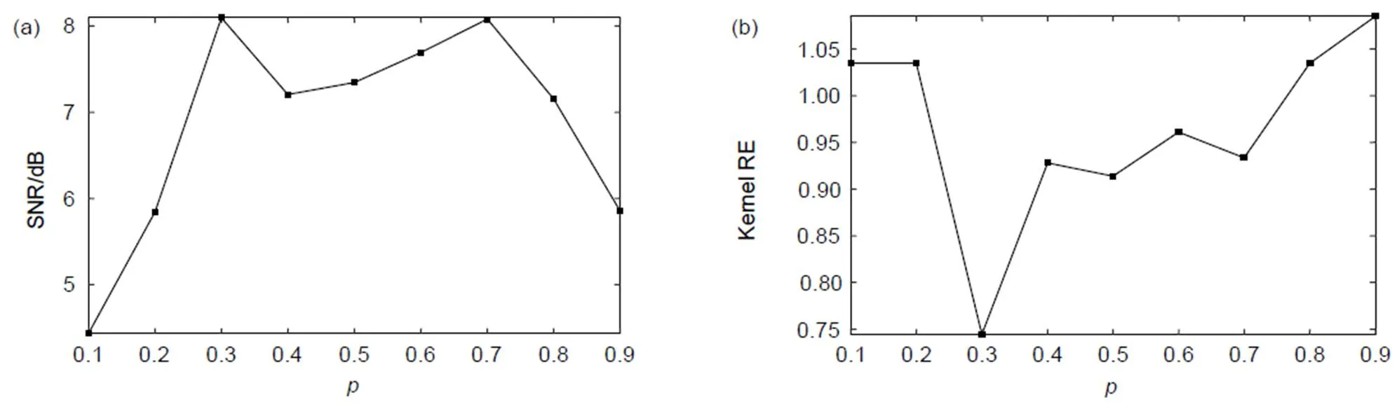
图5 不同p值下的复原图像SNRs和核估计误差RE

3.3 真实湍流退化图像复原

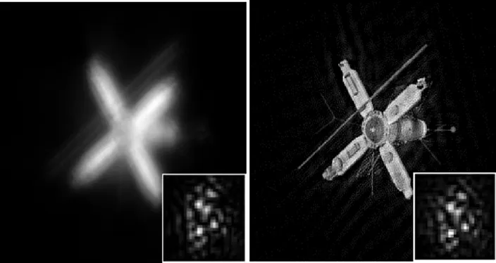
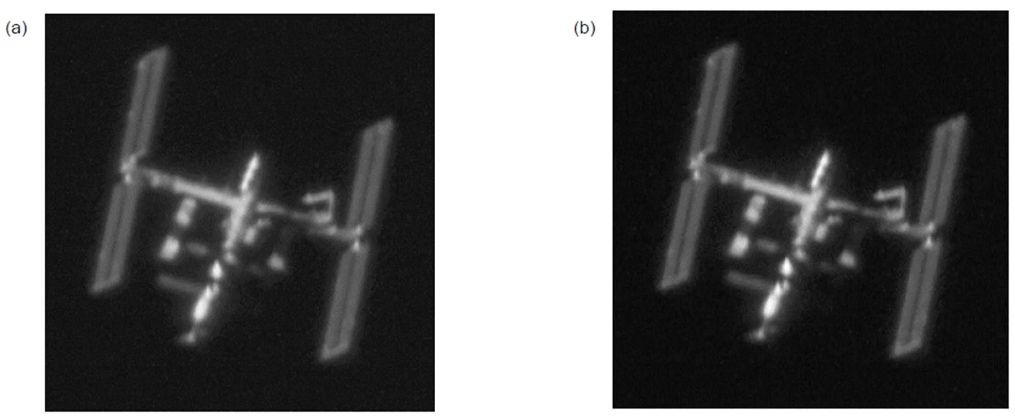
真实退化图像(图6(a))为口径80 cm的Munin望远镜采集到的国际空间站(International Space Station, ISS)图像，采集时间为2007年8月1日(来自www.tracking-station.de/images/images.html)。受大气湍流影响，图像明显降质，同时还含有大量噪声。分别使用总变分盲复原、稀疏先验=0.5和稀疏先验=0.1进行复原重建。可以看出前者(图6(b))的图像质量并未显著改善，而稀疏先验=0.5时(图6(c))，空间站的太阳能板的边缘更加清晰，其细节部分得到增强。而当的取值过小(=0.1)时，复原图像(图6(d))伴随着显著的噪声放大。图6(e)中分别给出了退化图像、总变分盲复原、稀疏先验=0.5和稀疏先验=0.1的复原图像的细节对比图。

4 结 论

图像总变分先验无法真实表征自然图像的梯度分布，盲去运动模糊常使用图像梯度的稀疏先验l(0<<1)来近似这种分布。本文将稀疏先验引入到大气湍流退化图像盲复原中，运用分裂Bregman算法和查表法求解稀疏导致的非凸代价函数，同时在非盲步骤中采用稀疏先验复原出锐利图像，避免了振铃现象。实验表明，与总变分先验相比，稀疏先验有利于模糊核的估计，降低了核估计误差，提升了复原质量。同时，值(0<<1)的选取不宜过大或过小，取值范围在[0.3，0.7]之间复原质量较高。最后，真实退化图像的复原结果表明了算法的有效性和稳定性。

[1] 姜文汉. 自适应光学技术[J]. 自然杂志, 2006, 28(1): 7–13.

Jiang W H. Adaptive optical technology[J]., 2006, 28(1): 7–13.

[2] Bao H, Rao C H, Tian Y,. Research progress on adaptive optical image post reconstruction[J].,2018, 45(3): 58–67.

鲍华, 饶长辉, 田雨, 等. 自适应光学图像事后重建技术研究进展[J]. 光电工程, 2018, 45(3): 58–67.

[3] Levin A, Weiss Y, Durand F,. Understanding and evaluating blind deconvolution algorithms[C]//, Miami, 2009: 1964–1971.

[4] Perrone D, Favaro P. Total variation blind deconvolution: the devil is in the details[C]//,Columbus,2014: 2909–2916.

[5] Ayers G R, Dainty J C. Iterative blind deconvolution method and its applications[J]., 1988, 13(7): 547–549.

[6] Lane R G. Blind deconvolution of speckle images[J]., 1992, 9(9): 1508–1514.

[7] Jefferies S M, Christou J C. Restoration of astronomical images by iterative blind deconvolution[J]., 1993, 415(2): 862–874.

[8] You Y L, Kaveh M. A regularization approach to joint blur identification and image restoration[J]., 1996, 5(3): 416–428.

[9] Chan T F, Wong C K. Total variation blind deconvolution[J]., 1998, 7(3): 370–375.

[10] Fergus R, Singh B, Hertzmann A,. Removing camera shake from a single photograph[J]., 2006, 25(3): 787–794.

[11] Krishnan D, Tay T, Fergus R. Blind deconvolution using a normalized sparsity measure[C]//, Providence, 2011: 233–240.

[12] Kotera J, Šroubek F, Milanfar P. Blind deconvolution using alternating maximum a posteriori estimation with heavy-tailed priors[C]//, York, 2013: 59–66.

[13] Goldstein T, Osher S. The split bregman method for L1-regularized problems[J]., 2009, 2(2): 323–343.

[14] Krishnan D, Fergus R. Fast image deconvolution using hyper-Laplacian priors[C]//, Vancouver, 2009: 1033–1041.

[15] Chan T F, Wong C K. Convergence of the alternating minimization algorithm for blind deconvolution[J]., 2000, 316(1–3): 259–285.

[16] Levin A, Fergus R, Durand F,. Image and depth from a conventional camera with a coded aperture[J].,2007, 26(3): 70.

[17] Wang Q T, Tong S F, Xu Y H. On simulation and verification of the atmospheric turbulent phase screen with Zernike polynomials[J]., 2013, 42(7): 1907–1911.王齐涛, 佟首峰, 徐友会. 采用Zernike多项式对大气湍流相位屏的仿真和验证[J]. 红外与激光工程, 2013, 42(7): 1907–1911.

Blind restoration of atmospheric turbulence degraded images by sparse prior model

Zhou Hairong1,2,3, Tian Yu1,2, Rao Changhui1,2*

1Key Laboratory of Adaptive Optics, Chinese Academy of Sciences, Chengdu, Sichuan 610209, China;2Institute of Optics and Electronics, Chinese Academy of Sciences, Chengdu, Sichuan 610209, China;3University of Chinese Academy of Sciences, Beijing 100049, China

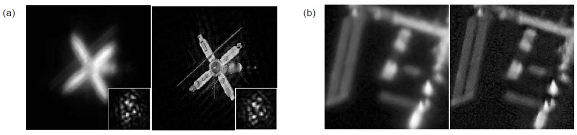
(a) Simulation: degraded and restoration; (b) Real observation: degraded and restoration

Overview:Atmospheric turbulence is a major factor limiting the imaging resolution of ground-based telescopes. Adaptive optics (AO) is commonly used to compensate for the wavefront distortion caused by turbulence to obtain higher resolution. However, due to the limitations of the system itself, such as the fitting error of the deformed mirror and the residual error caused by the time bandwidth, the closed-loop image still has residual errors, thus AO postprocessing technique is needed to further improve the image quality.

Blind deconvolution (BD) could recover a sharp image only from several degraded images. However, BD problems have the difficulties of ill-conditioned and infinite solutions, it is necessary to add prior knowledge to avoid undesired solutions. Traditional Wiener filtering based iterative blind deconvolution method assumes that the intensity of the image obeys the Gaussian distribution, while Chan et al. employ total variation prior, which assumes the gradient of the image obeys the Laplacian distribution. Given the fact that the gradient distribution of natural images is a sparse one with heavy tails, both of Gaussian and Laplacian model cannot approximate this sparse model greatly. Therefore, this paper draws on the image gradient sparse priori derived from blind motion deblurring, and applied it to the blind restoration of turbulence-degraded images.

In order to cope with the non-convex cost function caused by sparse prior, this paper uses split Bregman and look-up table method to solve effectively. Secondly, a two-step estimation strategy is adopted including kernel estimation and non-blind restoration. This paper employs the deconvolution method of Krishnan to reconstruct a sharp image with the kernel from the former step, and this strategy is essential to avoid the ringing effect reported by Fergus.

Firstly, the simulation experiment is carried out. To model the atmospheric turbulence degradation, the Zernike polynomials are used to generate the point spread function, and the OCNR5 satellite image is used as an object for observing. This paper adopts the relative error to evaluate the kernel estimation error and the signal to noise ratio (SNR) to evaluate image quality of degraded and restored ones. Both simulations and experiments on the real degraded images show that: 1) compared with the traditional Wiener filtering method and total variation prior, the sparse prior is beneficial to kernel estimation, produces sharp edges and removes ringing, thus improving the restoration quality. 2) After employing split Bregman optimization, restoration with sparse prior can converge rapidly and steadily, hence the proposed algorithm in this paper is robust and stable. 3) It is worth noting that the value ofshould not be too large or too small, smallerwill amplify the noise.

Citation: Zhou H R, Tian Y, Rao C H. Blind restoration of atmospheric turbulence degraded images by sparse prior model[J]., 2020, 47(7): 190040

Blind restoration of atmospheric turbulence degraded images by sparse prior model

Zhou Hairong1,2,3, Tian Yu1,2, Rao Changhui1,2*

1Key Laboratory of Adaptive Optics, Chinese Academy of Sciences, Chengdu, Sichuan 610209, China;2Institute of Optics and Electronics, Chinese Academy of Sciences, Chengdu, Sichuan 610209, China;3University of Chinese Academy of Sciences, Beijing 100049, China

Blind image deconvolution is one method of restoring both kernel and real sharp image only from degraded images, due to its illness, image priors are necessarily applied to constrain the solution. Given the fact that traditional image gradient2and1norm priors cannot describe the gradient distribution of natural images, in this paper, the image sparse prior is applied to the restoration of single-frame atmospheric turbulence degraded images. Kernel estimation is performed first, followed by non-blind restoration and the split Bregman algorithm is used to solve the non-convex cost function. Simulation results show that compared with total variation priori, sparse priori is better at kernel estimation, producing sharp edges and removal of ringing, etc., which reducing the kernel estimation error and improving restoration quality. Finally, the real turbulence-degraded images are restored.

adaptive optics; sparse prior; blind deconvolution; split Bregman

TP391

A

10.12086/oee.2020.190040

: Zhou H R, Tian Y, Rao C H. Blind restoration of atmospheric turbulence degraded images by sparse prior model[J]., 2020,47(7): 190040

周海蓉，田雨，饶长辉. 稀疏先验型的大气湍流退化图像盲复原[J]. 光电工程，2020，47(7): 190040

Supported by National Natural Science Foundation of China (11727805, 11703029)

* E-mail: chrao@ioe.ac.cn

2019-01-24；

2019-03-15

国家自然科学基金资助项目(11727805，11703029)

周海蓉(1994-)，女，硕士，主要从事自适应光学图像盲复原的研究。E-mail：zhouhairongwhu@foxmail.com

饶长辉(1971-)，男，博士，研究员，主要从事大口径高分辨力光学成像望远镜技术和系统研制工作。E-mail：chrao@ioe.ac.cn