Jinguo ZHANG (张金国)

School of Mathematics, Jiangxi Normal University, Nanchang 330022, China E-mail: jgzhang@jxnu.edu.cn

Tsing-San HSU (许清山) †

Center for General Education, Chang Gung University, Tao-Yuan, Taiwan, China E-mail: tshsu@mail.cgu.edu.tw

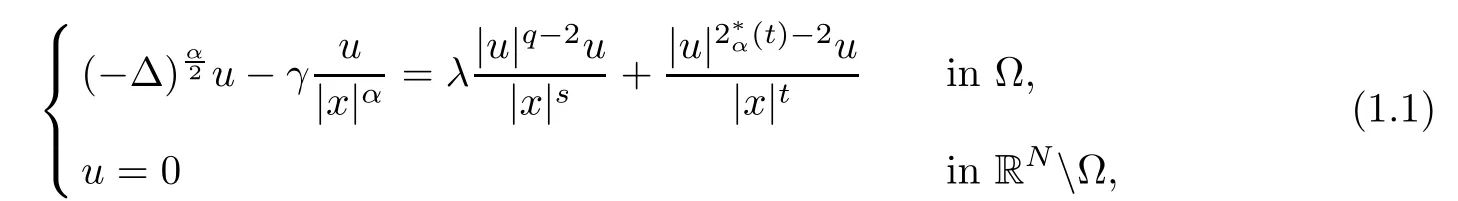
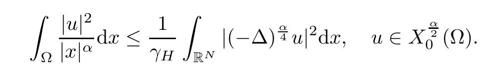
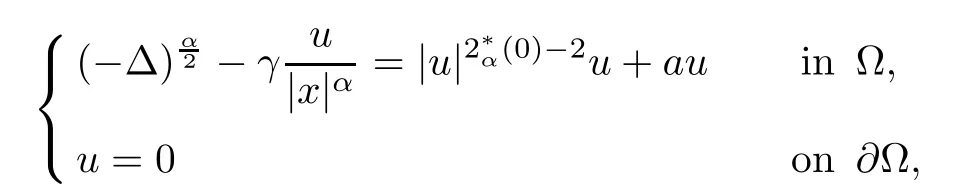
Abstract In this article, we study the following critical problem involving the fractional Laplacian: where Ω ⊂RN (N > α) is a bounded smooth domain containing the origin, α ∈(0,2),0 ≤s, t < α, 1 ≤q < 2, λ > is the fractional critical Sobolev-Hardy exponent, 0 ≤γ＜γH, and γH is the sharp constant of the Sobolev-Hardy inequality. We deal with the existence of multiple solutions for the above problem by means of variational methods and analytic techniques.

Key words Fractional Laplacian; Hardy potential; multiple positive solutions; critical Sobolev-Hardy exponent

1 Introduction

In this article, we are concerned with the existence and multiplicity of positive solutions for the following nonlocal elliptic problem with Hardy potential:

and endowed with the following norm

It is well-known that,if α=2,the operatoris defined aswhich is a local operator. The general problem

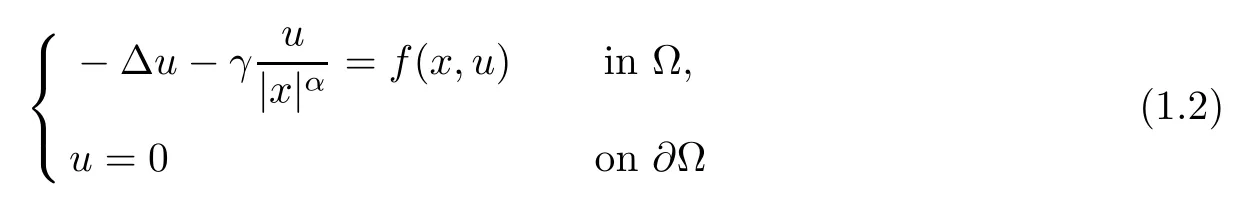
has been studied extensively. In case of γ = 0, Bahri-Coron [1] obtained the existence and multiplicity results for solutions of problem (1.2) with f(x,u) = |u|2∗−2u, and Passaseo [21]proved that problem (1.2) admits at least two weak solutions in(Ω). In the case ofwe recall that the existence of solutions for problem (1.1) has been obtained under different hypotheses on f(x,u); see Cao-Han [6], Chen [5], A. Ferrero, F. Gazzola [15], Smets [22],Terracini [27], Cao-Kang [8], Filippucci et al [17], and the references therein.

In this article, our main focus is on the case when 0 < α < 2. For these values of α, the operator is defined as

Existence of nontrivial solution for nonlinear elliptic equations with Hardy potential and fractional Laplace operator was recently studied by several authors;see[4,13,14,18,24,25,28–30] and the reference therein. For example, Yang and Yu [30] studied the following nonlocal elliptic problems with Dirichlet boundary condition

where α ∈(0,2), Ω ⊂RN(N >α) is an open bounded smooth domain with 0 ∈Ω, and a>0 is a constant. Moreover,in [14], Fall and Felli considered the unique continuation property and local asymptotic of solutions for the fractional elliptic problems with Hardy potential.

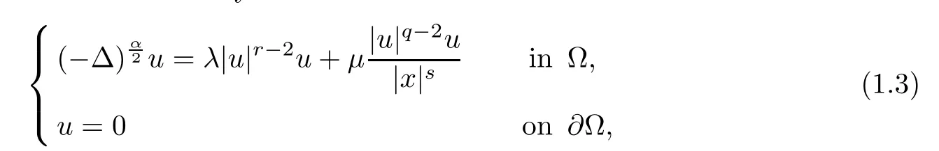
The starting point of this article is the result obtained by Shakerian [24]. Assuming that f(x) and g(x) are possibly change sign in, λ > 0, 0 ≤γ < γH, and 1 < q < 2 < p ≤(s),he proved in [24] that the problem

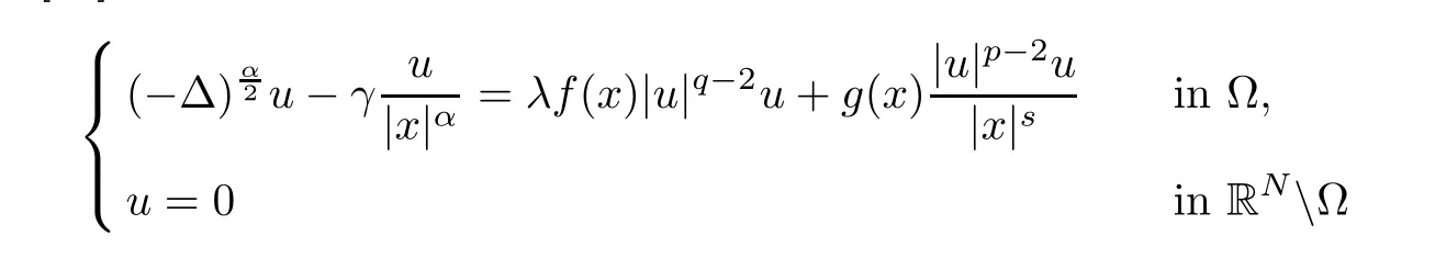
has at least two positive solutions for λ>0 sufficiently small.

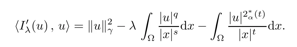
By refining and completing the analysis performed in [24], our goal is to obtain the existence and multiplicity of positive solutions for problem (1.1) in. As our methods are variational in nature, for any u ∈, we define the energy functionalassociated to (1.1) by

Much attention has been recently paid to the following limiting problem

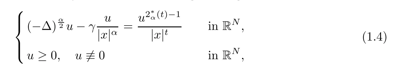
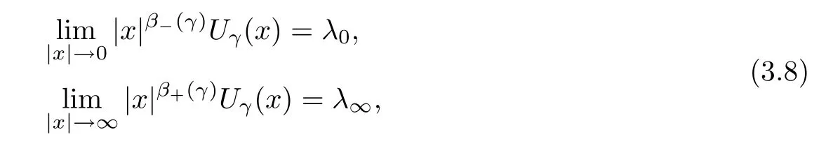
where 0 < α <2, 0 ≤t < α < N, and γ < γH. Ghoussoub-Shakerian [19] considered problem(1.4) and proved that if either 0 < γ < γHor {γ = 0 and 0 < t < α}, the equation has positive, radially symmetric, radially decreasing ground states, and which approaches zero as|x|→∞. Unlike the case of the Laplacian, no explicit formula is known for this ground states solution,but Ghoussoub et al[18]proved that any ground state solution u ∈Hα2(RN)satisfying u ∈C1(RN{0}) and

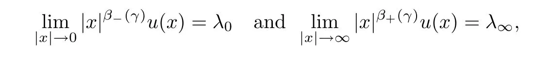
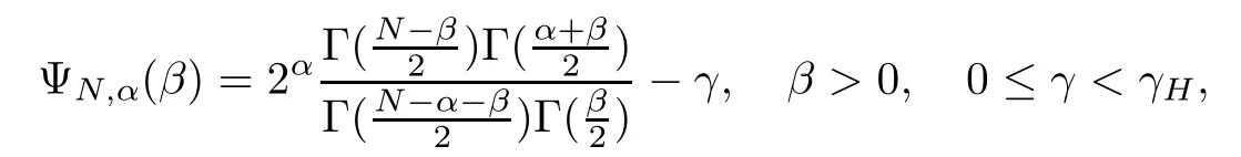
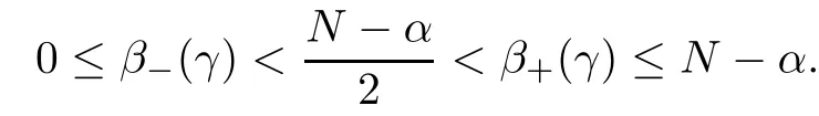
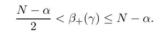
where λ0, λ∞> 0 and β−(γ) (resp., β+(γ)) is the unique solution in(resp., inof the following equation

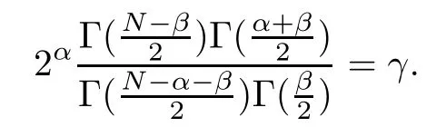
In particular, there exists C1, C2>0 such that

This article is devoted to the existence and multiplicity of solutions for the nonlocal elliptic problem(1.1)involving fractional critical Soboev-Hardy exponents and concave-convex nonlinearities. As no explicit formula is known for the ground state solution of the limiting problem(1.4), the critical case is more challenging and requires information about the asymptotic of this solutions at zero and infinity. We will get around the difficulty by working with certain asymptotic estimates for this ground state solution.

We are now ready to state our main results.

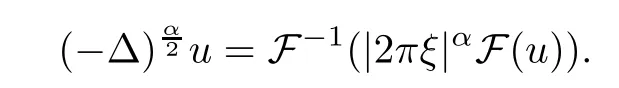
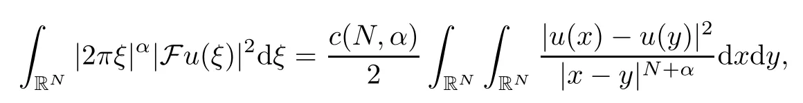
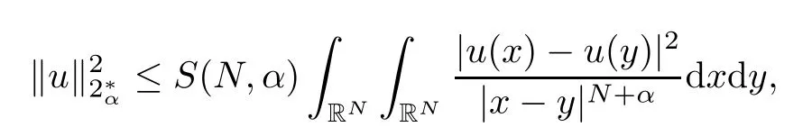
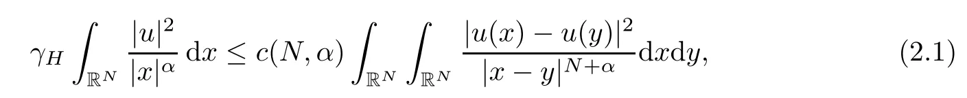
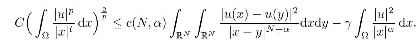
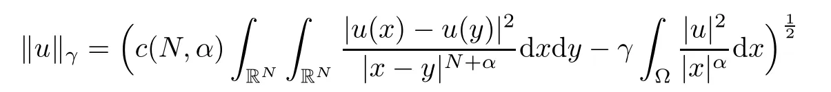
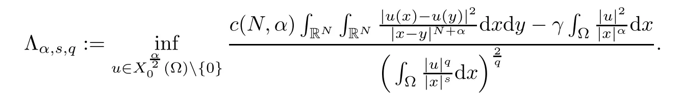
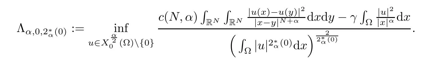
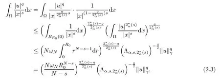
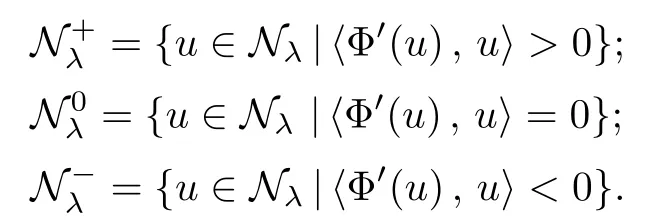
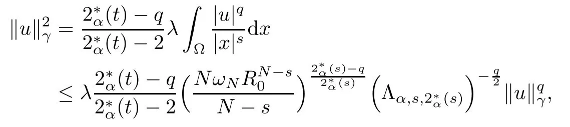
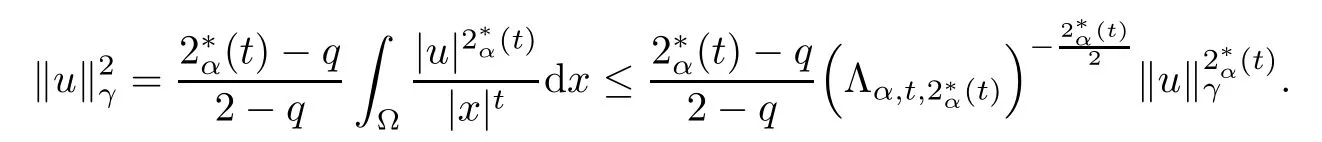
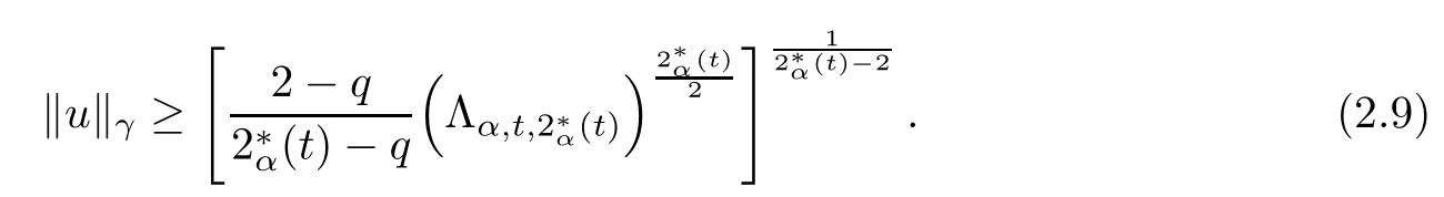
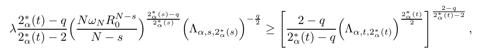
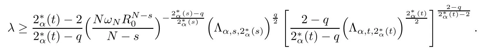
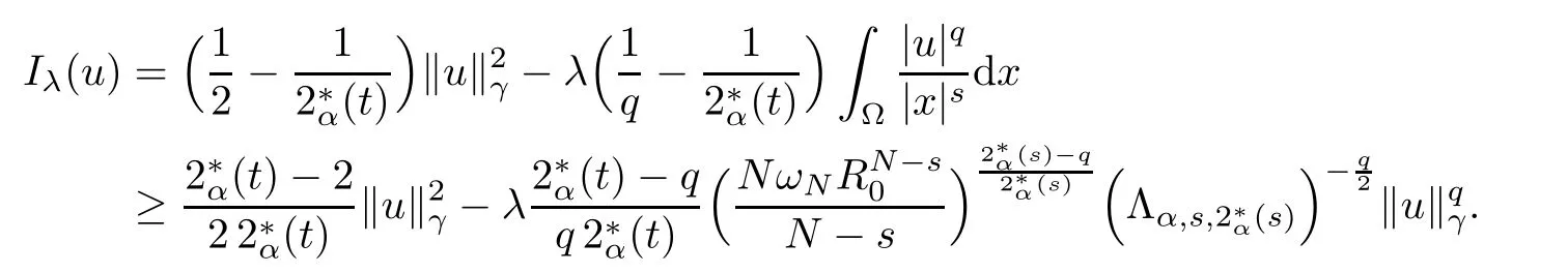
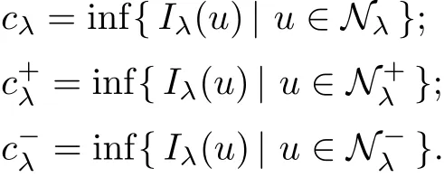
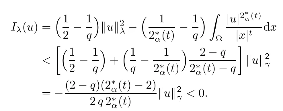
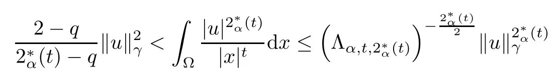
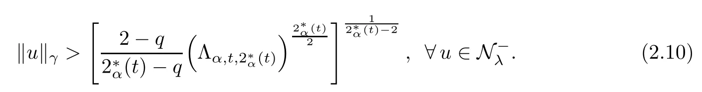
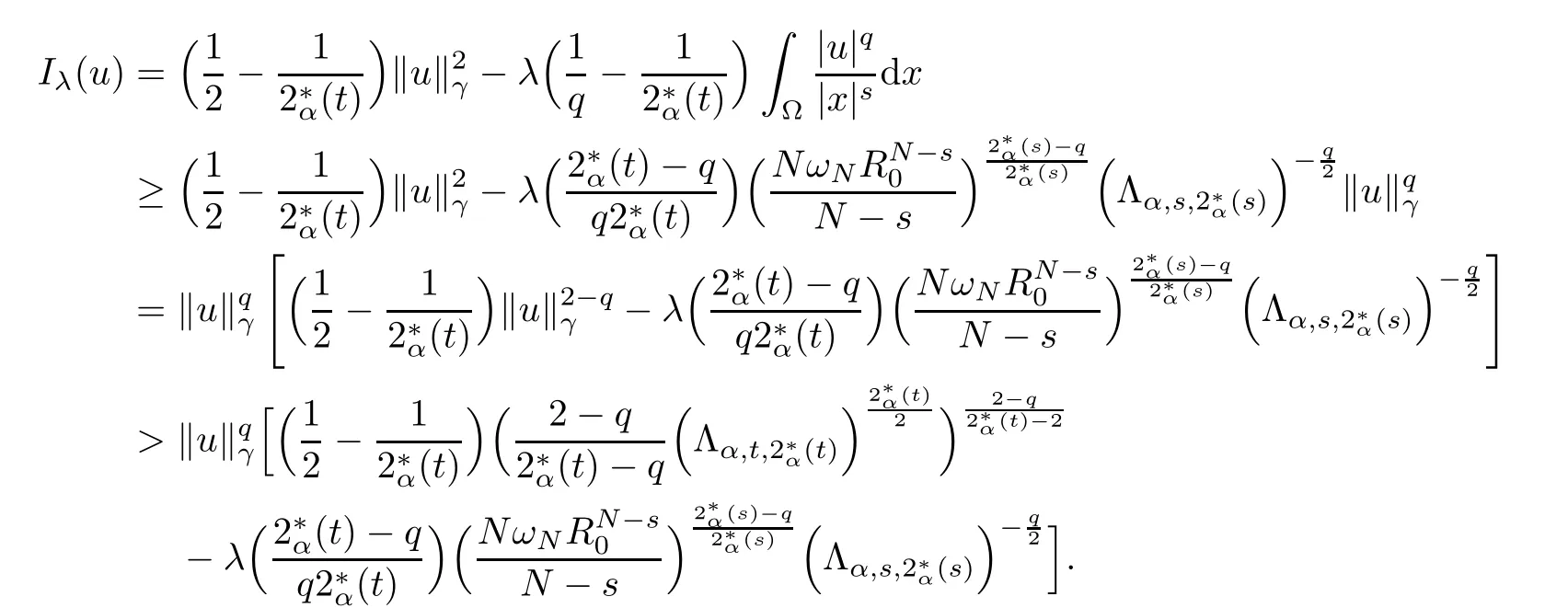
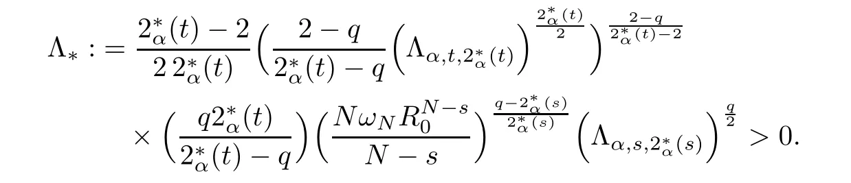
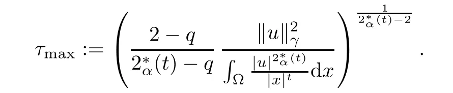
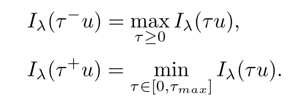
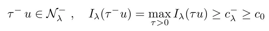
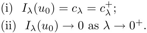
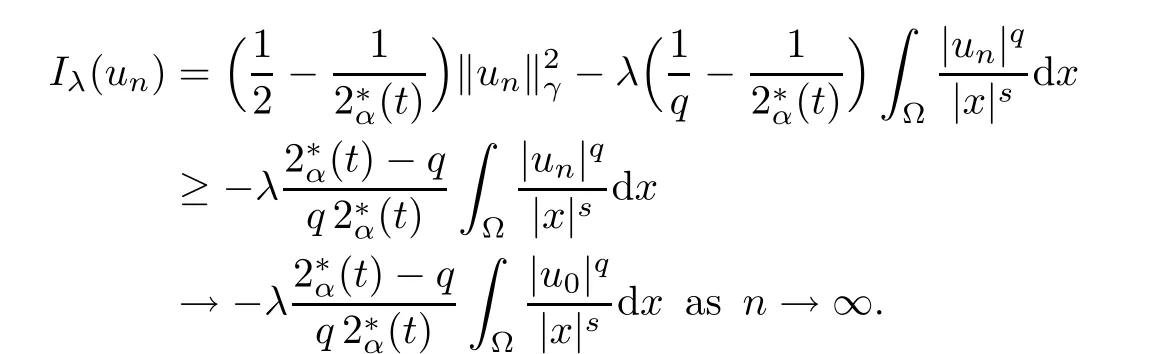
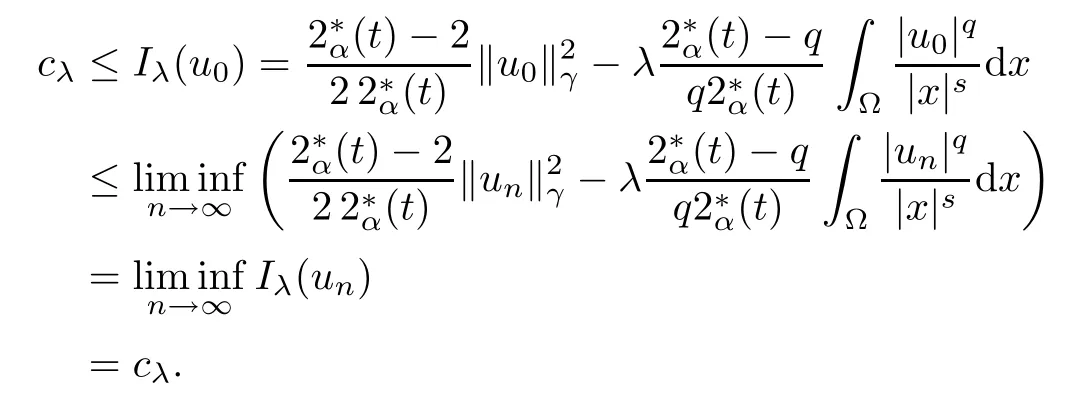
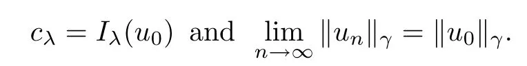
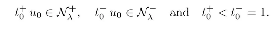
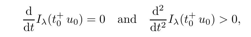
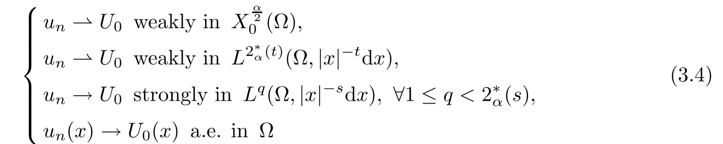
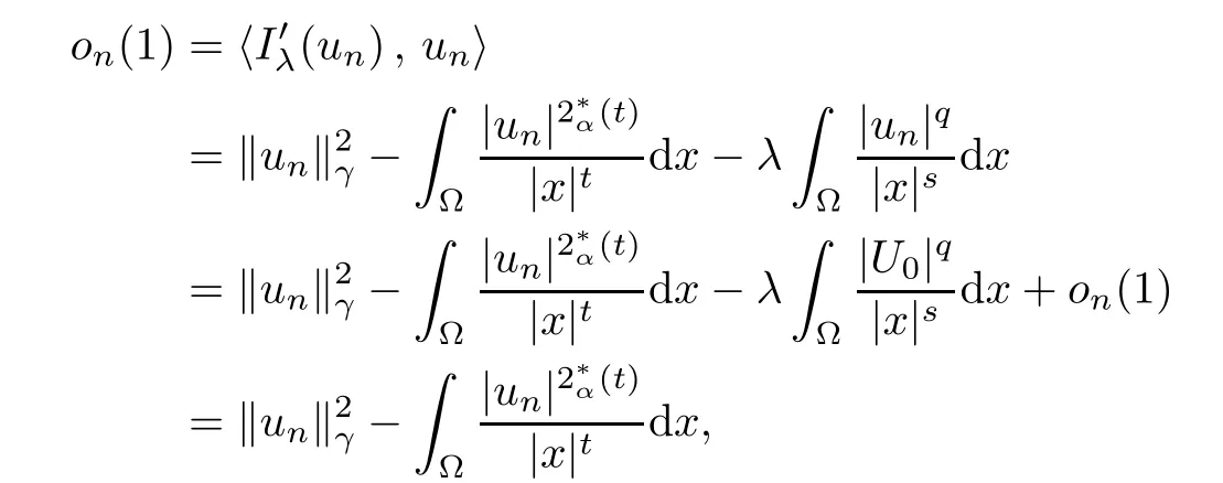
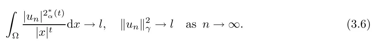
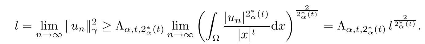
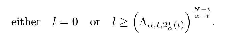
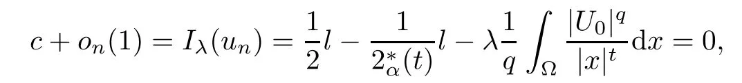
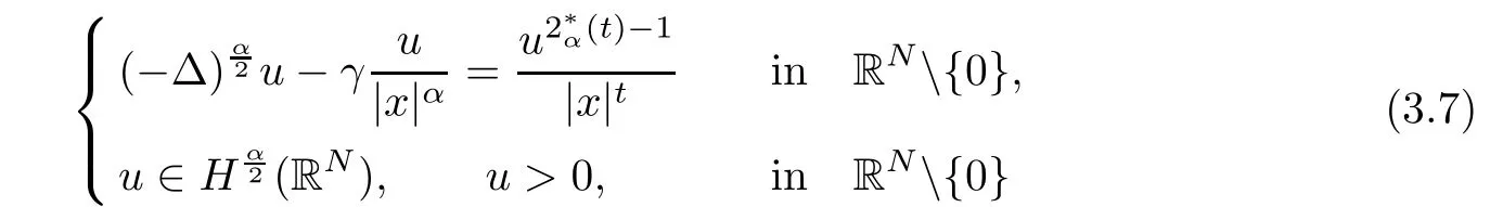
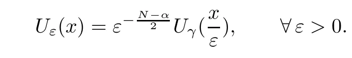
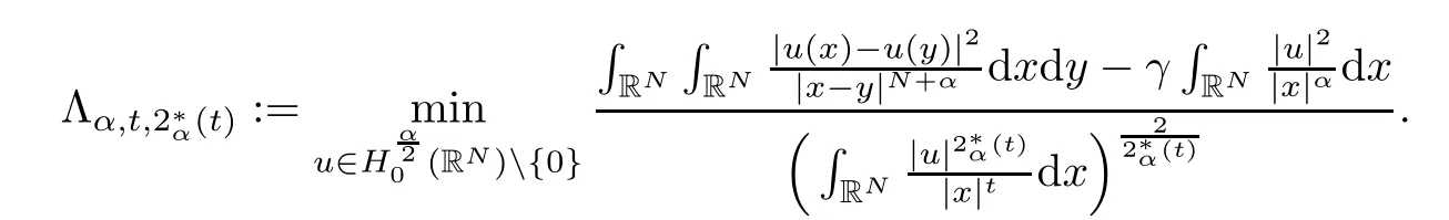
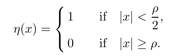
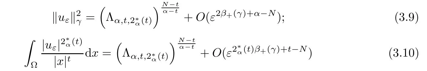
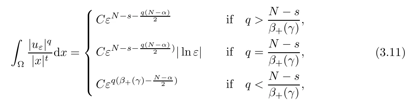
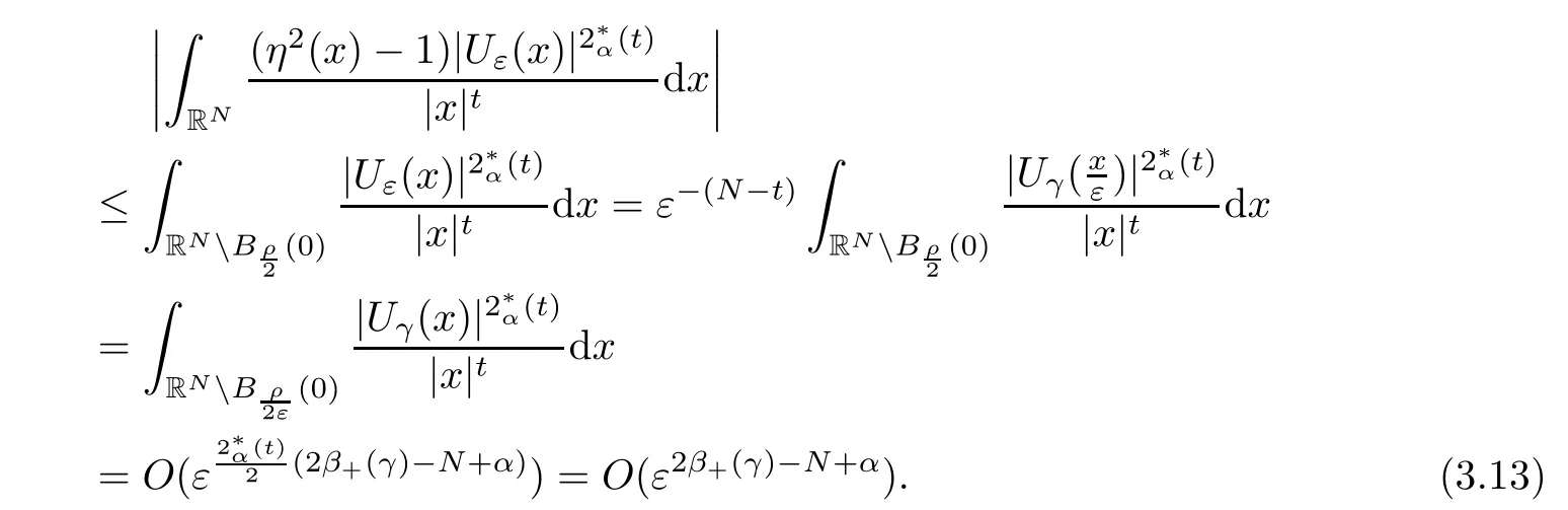
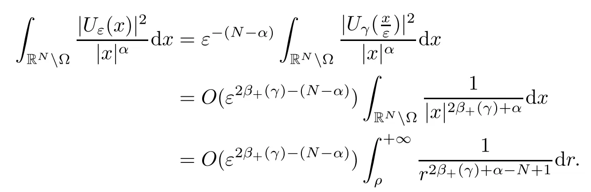
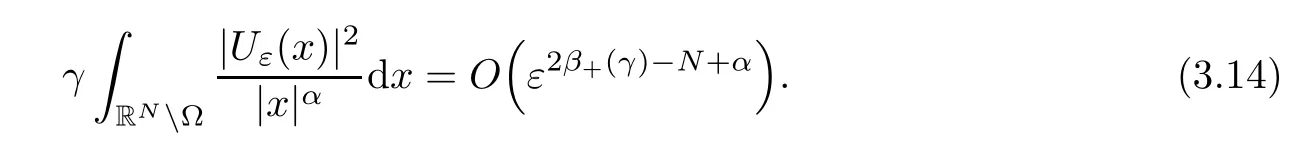
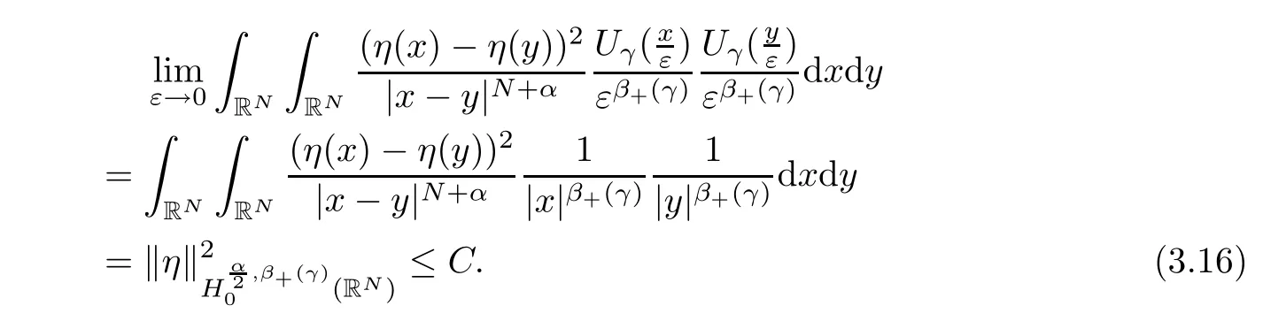
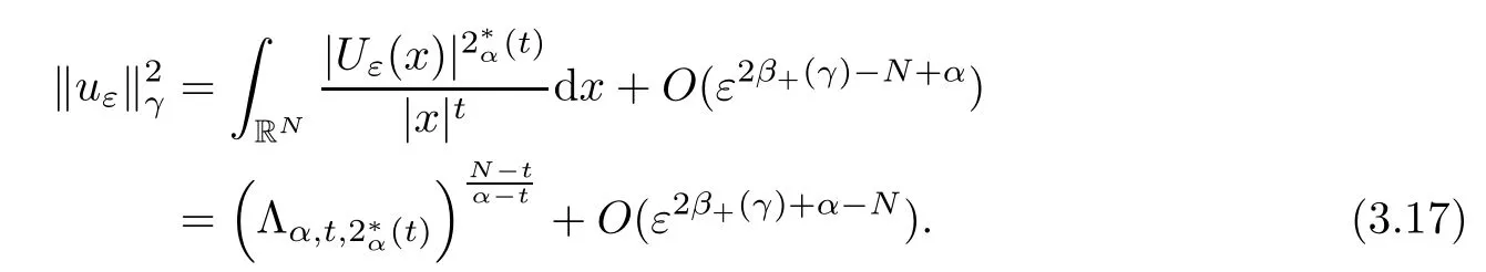
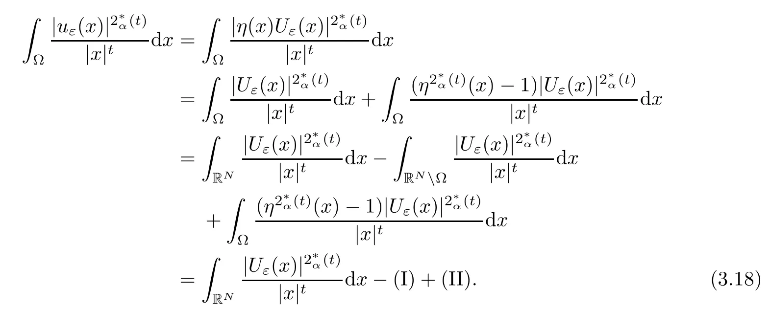
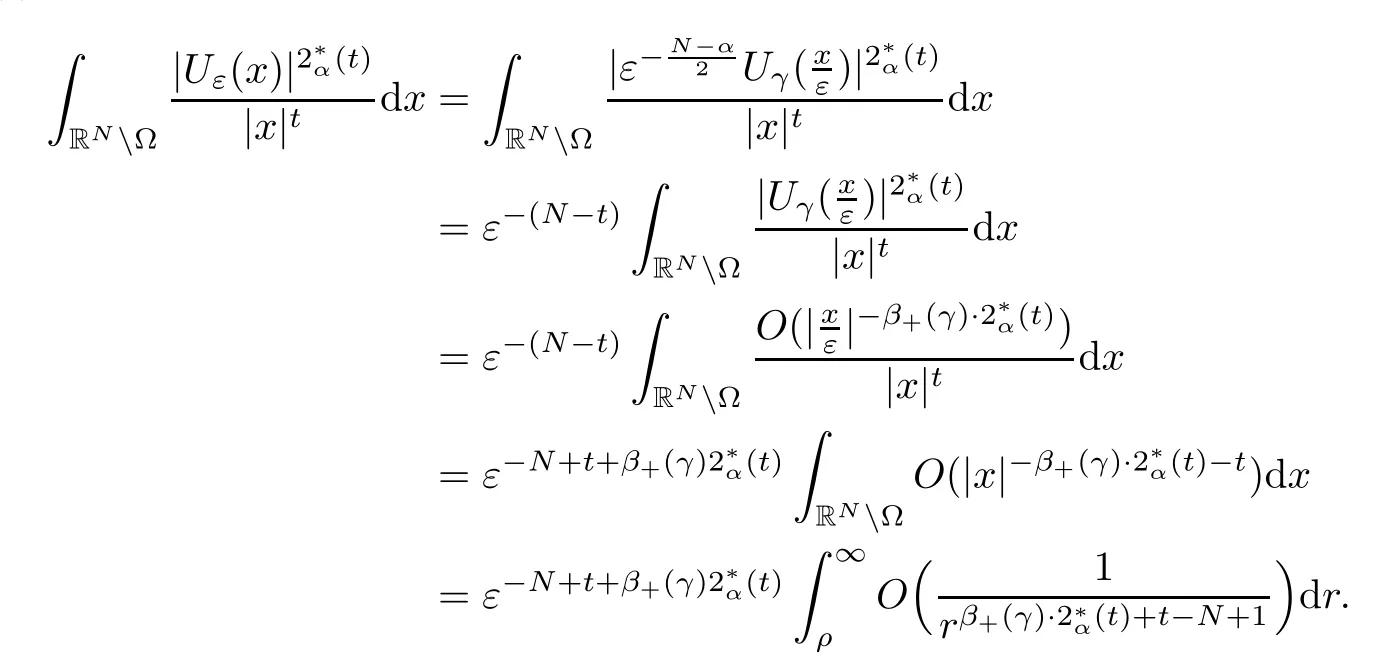
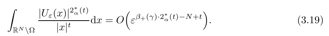
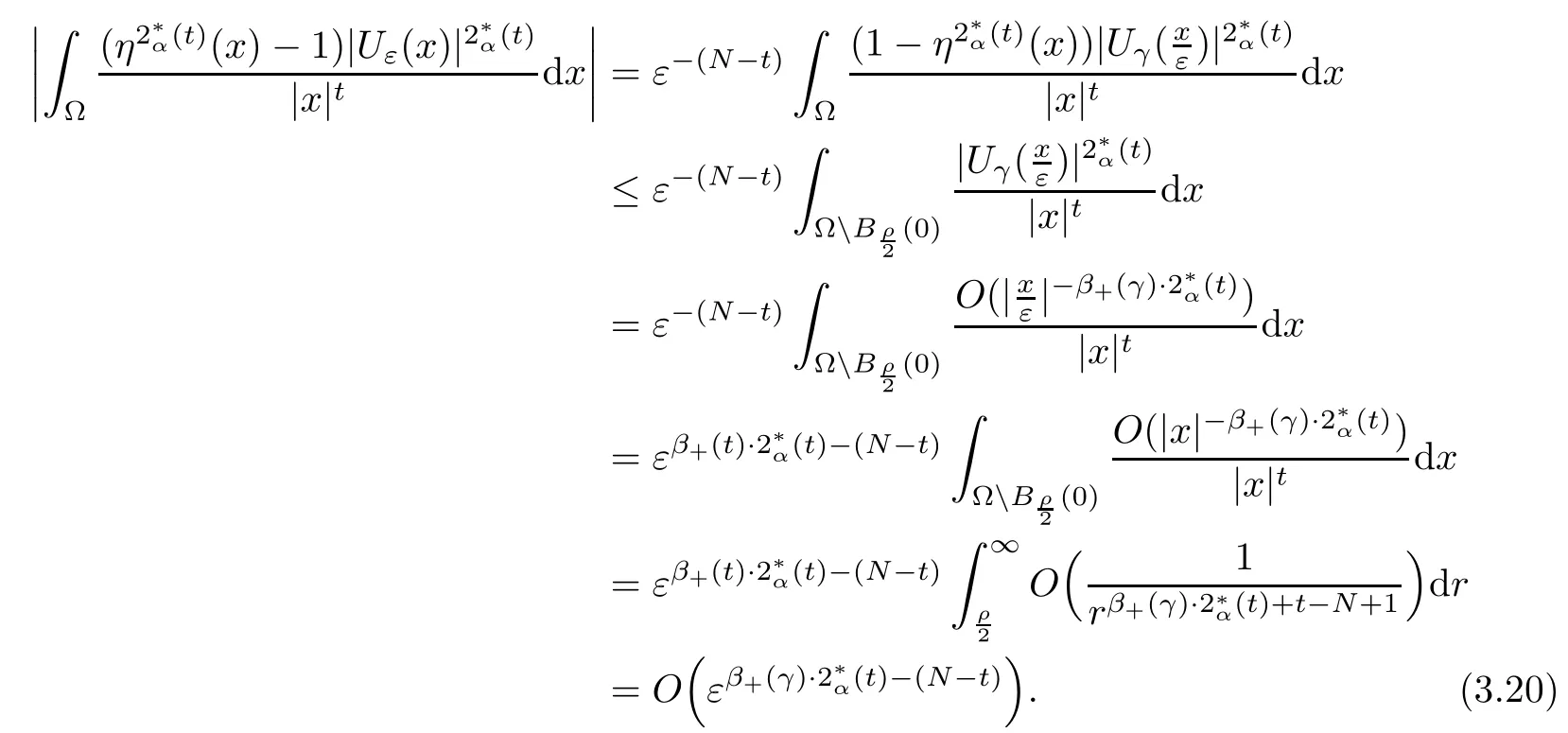
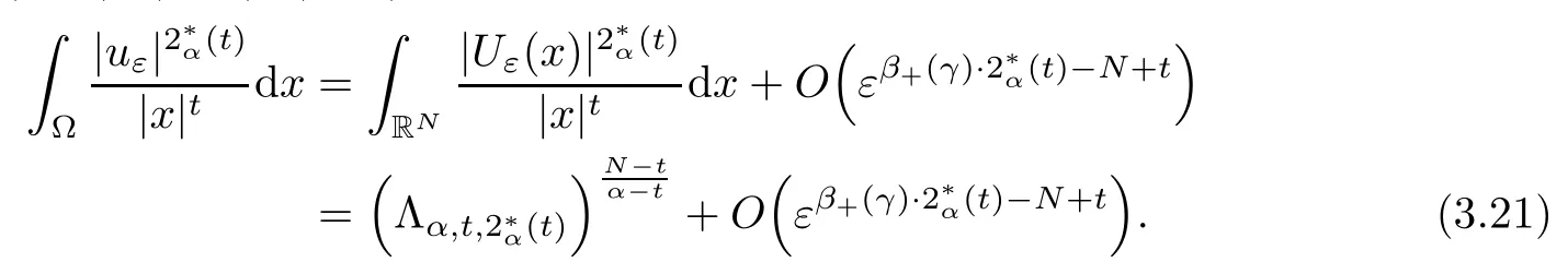
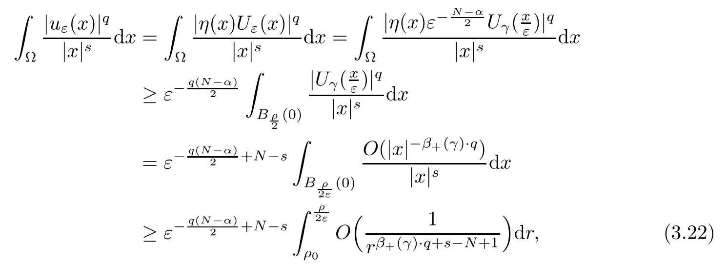
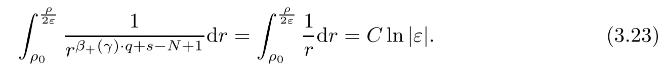
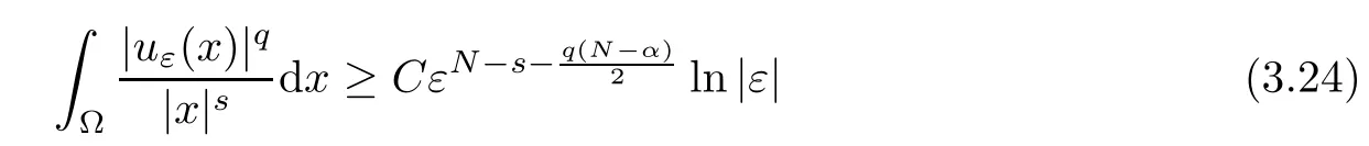
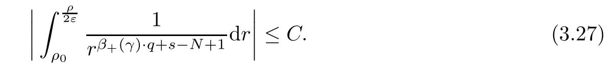
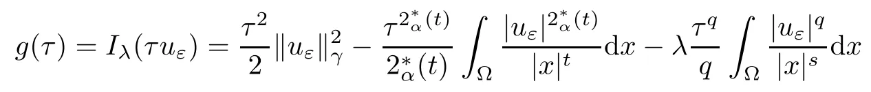
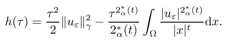
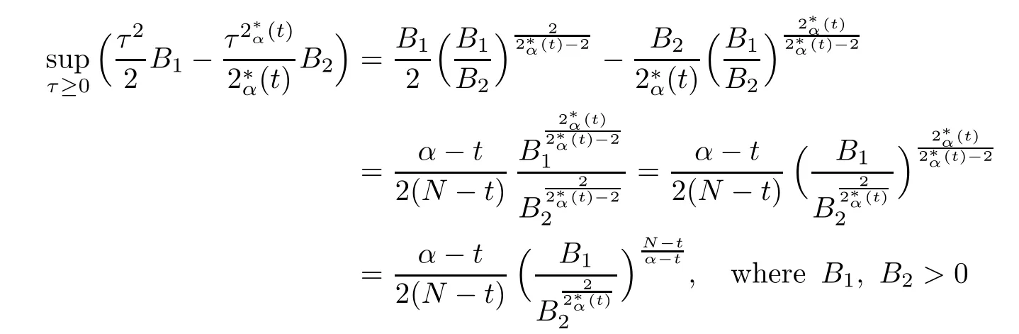
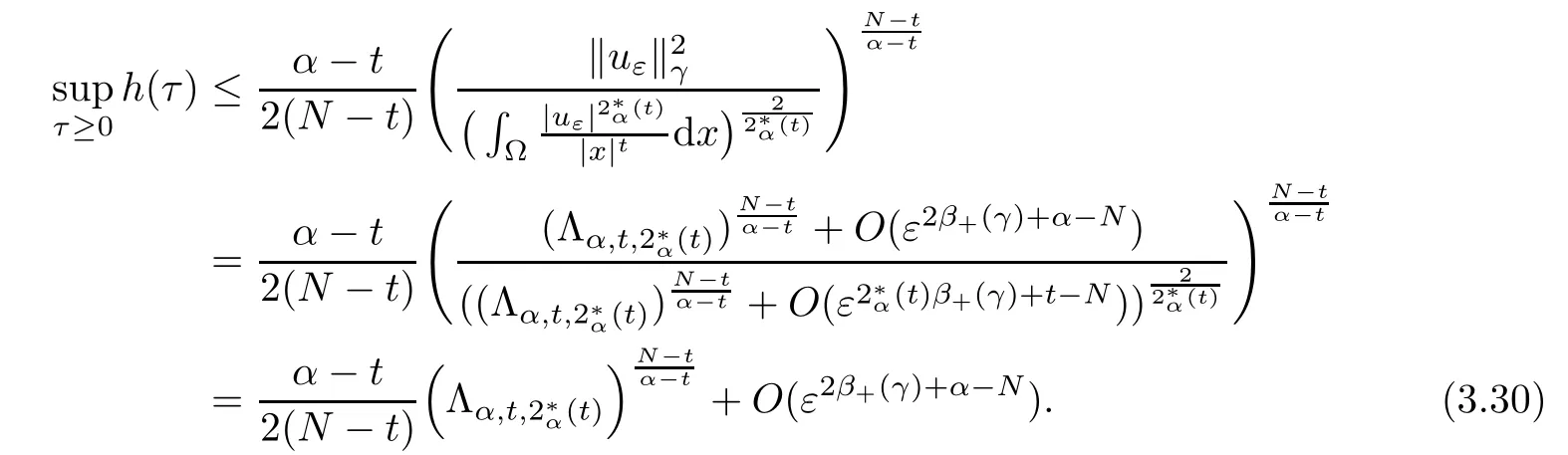
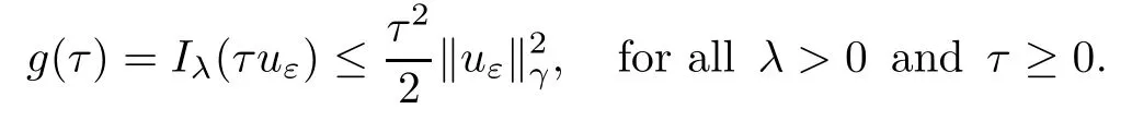
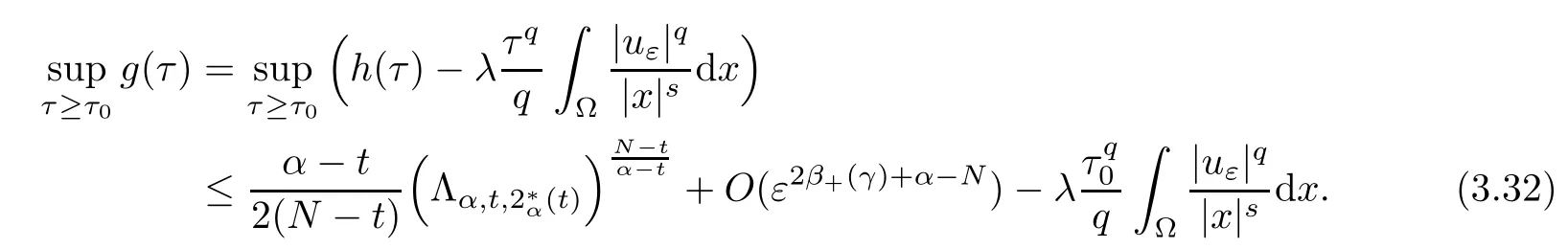
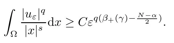
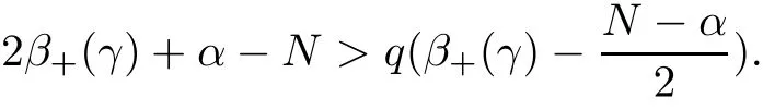
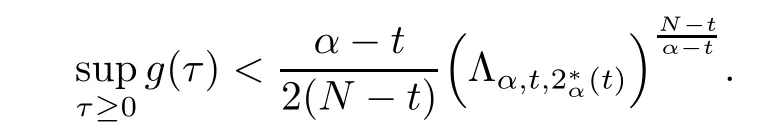
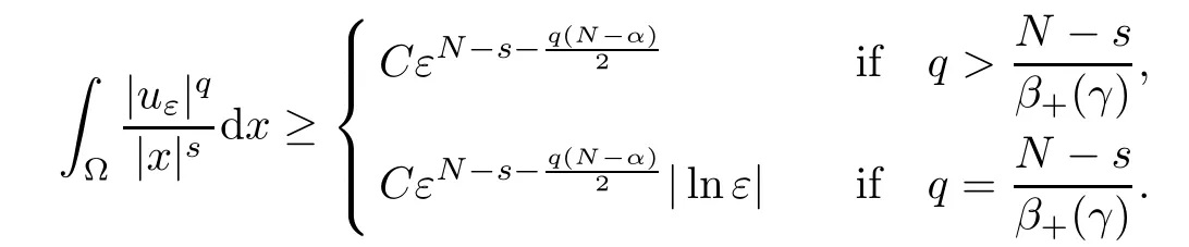
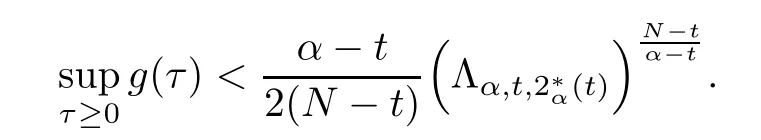
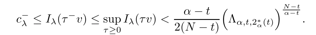
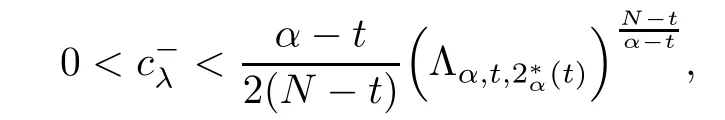
Theorem 1.1Assume that 0<α<2, N >α, 0 ≤γ <γH, 0

Then, we have the following results:

(1) There exists Λ0> 0, such that problem (1.1) has at least one positive solution for all λ ∈(0,Λ0).

(2) There exists Λ∗>0, such that problem (1.1) has at least two positive solutions for all λ ∈(0,Λ∗).

We prove Theorem 1.1 by critical point theory. However,the functional Iλdoes not satisfy Palais-Smale (PS) condition because of the lack of compactness of the embedding(Ω,|x|−tdx), so the standard variational argument is not applicable directly. In order to construct suitable Palais-Smale compact sequences, we need to locate the energy range where Iλsatisfies the Palais-Smale condition. By variational methods and analytic techniques, the existence and multiplicity of positive solutions to the problem is established. The conclusion are new for the elliptic equation with Hardy potential and fractional Laplacian operator.

This article is organized as follows. In Section 2,we give some preliminaries about fractional Laplacian and some properties of Nehari manifold. In Section 3, we complete the proof of Theorem 1.1. Throughout this article, we shall denote various positive constants as C. O(εt)denotesand o(εt) meansas ε →0. Lq(Ω,|x|−sdx) denotes the usual weighted Lq(Ω)space with the weight|x|−s. By o(1)we always means it is a generic infinitesimal value.

2 Notations and Preliminaries

In this section,we first introduce suitable function spaces for the variational principles that will be needed in the sequel, and give some properties of Nehari manifold.

2.1 The best constants Λα,s,q and Λα,0

First, we conclude the definitions of the best constants Λα,s,qand Λα,0. To continue, we recall the properties ofon the whole of RN, where it can be defined on the Schwartz class S (the space of rapidly decaying C∞functions on RN) via the Fourier transform,

Here, F(u) is the Fourier transform of u,. See [3, 12, 26] and references therein for the basics on the fractional Laplacian. Moreover,Caffarelli and Silvestre[9] introduced the α-harmonic extension to define the fractional Laplacian operator, and gave a new formulation of the fractional Laplacian through Dirichlet-to-Neumann maps. This is commonly used in the recent literature because it allows us to write nonlocal problems in a local way, and permits us to use the variational methods to solve those kinds of problems.Several results of the fractional version of the classical elliptic problems were obtained; we would like to mention [2, 7, 11, 31, 32] and the references therein.

For 0 < α < 2, the fractional Sobolev spaceis defined as the completion of(RN) under the norm

By Proposition 3.6 in [12], for all, the following relation holds:

We start with the fractional Sobolev inequality [10], which asserts that for N > α and α ∈(0,2), there exists a constant S(N,α)>0 such that

By interpolating these inequalities via Hölder’s inequalities,one gets the following fractional Sobolev-Hardy inequality [19].

Lemma 2.1Assume that 0<α <2, 0 ≤t<α

Let now Ω ⊂RNbe a bounded domain, and we define the spaceas

with the norm and the scalar product as follows:

Remark 2.2Under the same conditions on α, t, p, and γ < γH, for any u ∈Lemma 2.1 shows that there exists a positive constant C such that

If γ <γH, it follows from (2.1) that

From the fractional Hardy inequality and fractional Sobolev-Hardy inequality, for 0 ≤γ <γH, 0 ≤s<α, and 2 ≤q ≤(s), we can defined the best fractional Sobolev-Hardy constant:

In what follows,without loss of generality,we may assume throughout this article that c(N,α)≡1.

Let R0be a positive constant such that Ω ⊂BR0(0),where BR0(0)={x ∈RN: |x|

By the Hölder and Sobolev-Hardy inequalities, for all u ∈, we get

2.2 Nehari manifold

We consider the problem on the Nehari manifold. Define the Nehari manifold:

where

Notice that Nλcontains all nonzero solutions of (1.1). Define

We split Nλinto three parts:

In order to prove our main results, we now present some important properties of,, and. The first result shows that minimizers on Nλare the critical point for Iλin

Lemma 2.3If u ∈(Ω)is a local minimizer for Iλon Nλand,thenin(Ω), where(Ω) is the dual space of

ProofIf u0is a local minimizer of Iλon Nλ, then there exists a neighborhood D of u0such that u0is a nontrivial solution of the optimization problem

Hence, by the theory of Lagrange multipliers, there exists θ ∈R such thatinwhich implies that

Lemma 2.4There exists a positive number Λ0>0 such that if λ ∈(0,Λ0),then

ProofArguing by contradiction, we assume that there exists a Λ0>0 such thatfor all λ ∈(0,Λ0). By (2.3) and (2.6), for any u ∈, we get

which implies that

On the other hand, from (2.3) and (2.5), we have

It follows that

Thus, it follows from (2.8) and (2.9) that

that is,

So, we get λ ≥Λ0. This is a contradiction. Here,

and completes the proof.

Lemma 2.5The energy functional Iλis coercive and bounded from below on Nλ.

ProofIf u ∈Nλ, then by (2.3), we obtain

For C >0, set

By Lemmas 2.4 and 2.5, for each λ ∈DΛ0, we get, and the energy functional Iλis coercive and bounded from below on Nλ,, and. Then, the Ekeland variational principle implies that Iλhas a minimizing sequence on each manifold of Nλ,, and.

Define

Lemma 2.6Assume that 0 < α < 2, N > α, 0 ≤γ < γH, 0 < s, t < α, and 1 ≤q < 2.

Then, we have the following results:

(i) cλ≤<0 for all λ ∈;

(ii) There exist c0, Λ∗>0 such that≥c0for all λ ∈, where

Proof(i) From the definition of cλand, we can deduce that cλ≤. Moreover, for u ∈, by (2.5), we get

and so

It follows that

This completes the proof.

Remark 2.7It is easy to verify that

Similar to Lemma 3.4 in [24], we can get the following result.

Lemma 2.8Assume that λ ∈DΛ0. Then, for anythere exist τ+,τ−>0 such that τ+<τmax<τ−, τ−u ∈, τ+u ∈, and

ProofThe proof is similar to [24, Lemma 3.4 ], and we omit the details here.

Remark 2.9By Lemmas 2.6(ii) and 2.8, for any u ∈(Ω){0}, we can easily deduce that there exist t−, c0>0 such that

3 Proof of the Main Results

In this section, we use the results in Section 2 to prove the existence of a positive solution on, as well as on. First, we state the following result.

Proposition 3.1(i) Assume that λ ∈. Then, there exists a minimizing sequence{un}⊂Nλfor Iλsuch that Iλ(un)→cλand(un)→0 as n →∞.

ProofThe proof is similar to [24, Proposition 3.8] and is omitted.

Theorem 3.2Assume that N > α, 0 ≤γ < γH, 0 ≤s, t < α, 1 ≤q < 2, and λ ∈DΛ0.Then, there exists u0∈such that u0is a positive solution of (1.1) and satisfy

ProofBy Proposition 3.1 (i), there exists a minimizing sequence {un}⊂Nλsuch that

From Lemma 2.5, {un} is bounded inThus, there is a subsequenceandsuch that

It follows that

By (3.1),(3.2),and(3.3), it is easy to prove that u0is a weak solution of (1.1). Moreover,from{un}⊂Nλand (3.3) , we obtain

This and Iλ(un) →cλ< 0 (see Lemma 2.6 (i)) yield that, that is,. As Iλ(u0) = Iλ(|u0|) and |u0| ∈Nλ, we may assume that u0is a nontrivial nonnegative solution of (1.1). Moreover, it follows from the strong maximum principle [23, Proposition 2.2.8] that u0>0 in Ω.

Now, we prove that un→u0strongly inand Iλ(u0) = cλ. By applying Fatou’s lemma and un, u0∈Nλ, we have

This implies that

Standard argument shows that un→u0strongly in

Next, we claim u0∈. Indeed, if u0∈, by Lemma 2.8, there exist uniqueand>0 such that

As

which contradicts Iλ(u0)=cλ. Consequently, u0∈.

Finally, it follows from (2.3) and Lemma 2.6 (i) that

This implies that Iλ(u0)→0 as λ →0+, and completes the proof.

In the following theorem, we prove the existence of a positive solution of (1.1) on N−λ .

In obtaining the existence result on N−λ , it is critical to have the (PS) conditions for all levelwhich will be shown in the next two results, seeing Lemmas 3.3 and 3.7.

Lemma 3.3Assume that N > α, 0 ≤γ < γH, 0 ≤s, t < α, and 1 ≤q < 2. If {un} is a (PS)c-sequence for Iλwith cthen there exists a subsequence of{un} converging weakly to a nonzero solution of (1.1).

ProofSuppose thatsatisfies Iλ(un) →c and I(un) →0 with c ∈As{un}is bounded in,passing to a subsequence if necessary,there existssuch that

Hence, from (3.4), it is easy to see that(U0)=0 and

Now, we claim that U0= 0. Arguing by contradiction, we assume U0≡0. By (3.4) and(3.5), as n →∞,

which implies

Then, from the definition of Λα,t,2∗α(t)and (3.6), we have

This implies

If l =0, then by (3.5) and (3.6), we get

which contradicts c>0. Thus, we conclude that. Hence,

This contradicts the assumption on c. Thus, U0is a nontrivial weak solution of (1.1).

Lemma 3.4(see [18, 19]) Assume that 0<α<2, 0

has positive,radially symmetric,radially decreasing ground statesthat satisfyand Uγ∈C1(RN{0}). Furthermore, Uγhas the following properties:

where λ0, λ∞are positive constants and β−(γ), β+(γ) are zeros of the function

and satisfy

In particular, there exists C1, C2>0 such that

Remark 3.5We know that the ground state Uγ(x) is unique up to scaling, that is, all ground state must be the form

Moreover, the critical level is given by, where

In addition, the ground state Uεsatisfy

Now,we will give some estimates on this ground state solution. Choose ρ>0 small enough such that Bρ(0)⊂Ω, η ∈(Ω), 0 ≤η(x)≤1, and

Set uε(x)=η(x)Uε(x). We get the following results.

Proposition 3.6Assume that 0 < α < 2, N > α, 0 ≤γ < γH, 0 ≤s, t < α, and 1 ≤q <(s). Then, as ε →0, we have the following estimates:

and

where the number β+(γ) is a solution of the equation ΨN,α(β)=0 and satisfy

ProofFor (3.9), we can compute

Using (3.8), it is easy to check that

Similarly, we have

Moreover,

It follows from Ground State Representation [16] and Legesgue’s convergence theorem that there exists C >0 such that

So, (3.12), (3.13), (3.14), (3.15), (3.16), and Remark 3.5 imply that

In order to get (3.10), we first compute

Now, we estimate last two terms in (3.18).

For (I), we have

For (II), we obtain

Therefore, from (3.18), (3.19), (3.20), and Remark 3.5, we get

Hence, this completes the proof of (3.10).

Finally, we compute (3.11). For all 1 ≤q <(s), as ε →0,

where the constant ρ0>0 is small enough.

(i) If β+(γ)·q+s −N =0, straightforward computations yield

So, (3.22) and (3.23) yield that

(ii) If β+(γ)·q+s −N <0, it follows that β+(γ)·q+s −N +1<1 and

Then, inserting (3.25) into (3.22), we obtain

(iii) If β+(γ)·q+s −N >0, we have β+(γ)·q+s −N +1>1, then there exists C > 0 such that

Therefore, by (3.22) and (3.27), we have

Thus, (3.24), (3.26), and (3.28) imply that (3.11) holds.

Lemma 3.7Assume that 0 < α < 2, 0 ≤γ < γH, 0 ≤s,t < α < N and 1 ≤q < 2.

Then, for all λ ∈DΛ0, there existssuch that

ProofLet Uγ(x) be a ground state solution of problem (3.7), ρ > 0 small enough such that Bρ(0) ⊂Ω. Let η ∈(Ω) be a cut-off function satisfying 0 ≤η(x) ≤1 , η(x) = 1 for|x|

and

By the fact that

and Proposition 3.6, we can get

On the other hand, using the definitions of g and uε, we get

Combining this with (3.9), let ε ∈(0,1), then there exists τ0∈(0,1)independent of ε>0 such that

Hence, for all λ>0 and 1 ≤q <2, by (3.30), we have

Now, we need to distinguish two cases:

Then

Combining this with (3.31)and(3.32), for all λ ∈,we can choose ε small enough such that

Therefore, from (3.31), (3.32), and (3.33), for all λ ∈, we can choose ε > 0 small enough such that

From cases (i) and (ii), (3.29) holds by taking v =uε.

From Lemma 2.8, Remark 2.9, the definition of, and(3.29), for any λ ∈, we obtain the result that there exists τ−>0 such that τ−v ∈and

Hence, the proof is thus completed.

Now, we establish the existence of a local minimum of Iλon.

Theorem 3.8Assume that 0<α<2, N >α, 0 ≤γ <γH, 0 ≤s, t<α, and 1 ≤q <2.Then, for any λ ∈DΛ∗, the functional has a minimizer U0inand satisfies the following:

(i) Iλ(U0)=λ;

(ii) U0is a positive solution of (1.1).

ProofFor all λ ∈,by Proposition 3.1(ii),there exists a minimizing sequence{un}⊂for Iλsuch that

Using Lemmas 2.6 (ii) and 3.7, we get the energy levelsatisfying

which and Lemma 2.5 imply that {un} is bounded in. From Lemma 3.3, there exists a subsequence still denoted by {un} and a nontrivial solutionsuch that un⇀U0weakly in

This is a contradiction. Consequently,

Next, by the same argument as that in Theorem 3.2, we get un→U0strongly inand=Iλ(U0) for all λ ∈. Moreover,from Iλ(|U0|)=Iλ(U0) and |U0|∈, then U0is a nontrivial nonnegative solution of (1.1).

Finally, by the maximum principle [23, Proposition 2.2.8], then U0is a positive solution of(1.1). The proof is complete.

Proof of Theorem 1.1The part (i) of Theorem 1.1 immediately follows from Theorem 3.2. When λ ∈DΛ∗, by Theorems 3.2 and 3.8, then (1.1) has at least two positive solutions u0and U0such that u0∈and U0∈. As, this implies that u0and U0are distince. This completes the proof of Theorem 1.1.