MA Xue-min, ZHANG Ling, LI Bao-lin

(1- Teaching Department of Science, Gansu University of Chinese Medicine, Dingxi, Gansu 743000;2- College of Mathematics and Information Science, Northwest Normal University, Lanzhou 730070)

Abstract: In this paper, by using the theories of Kurzweil integral and bounded Φ-variation function.Emphatic convergence for Kurzweil equations and its application for a sequence of ordinary differential equations are discussed.The theorem of emphatic convergence for bounded Φ-variation solutions of Kurzweil equations is obtained.The result is continuation of continuous dependence of bounded Φ-variation solutions on parameters for Kurzweil equations and essential generalization of the emphatic convergence for bounded variation solutions of Kurzweil equations.

Keywords: Kurzweil equations; emphatic convergence; bounded Φ-variation function

1 Introduction

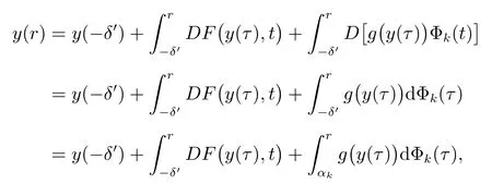
Kurzweil equations were introduced in 1957 by Kurzweil.The theory of Kurzweil equations have been proved to be useful in dealing with the continuous dependence on parameter for differential equations, measure differential equations and systems with impulses, volterra integral equations and topological dynamics[1-8].For a detailed discussion of this equations, see [9–12].In [12], Li and Wu considered continuous dependence of bounded Φ-variation solutions on parameters for the following Kurzweil equations

Throughout the paper, the following notations will be used.

Assume that G = Bc× (a,b), Bc= {x ∈ Rn;||x|| < c}, c > 0.−∞ < a < b <+∞, F(x,t):G → Rnis an Rn-valued function defined.

This paper is organized as follows: in next section, we show some basic definitions,key lemmas and theorem.In section 3, we get the theorem of emphatic convergence for bounded Φ-variation solutions of Kurzweil equations.In the final section, the application for a sequence of ordinary differential equations is discussed.

2 Preliminaries

In this section, we will show some basic definitions, key lemma and theorem.Let’s start with the definition of Kurzweil integral which plays a crucial pole in the theory of Kurzweil equations.

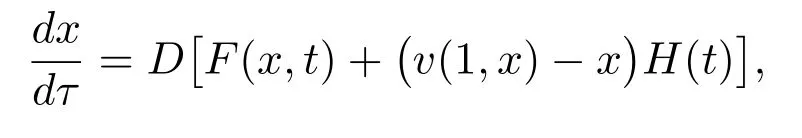
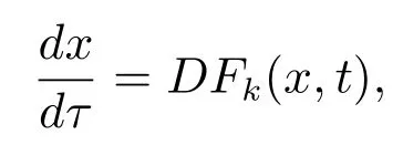
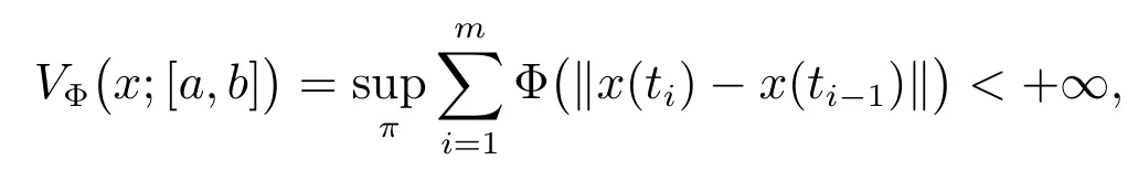
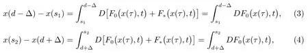
Definition 1[4,10-12]A function U : [a,b]× [a,b]→ Rnis said to be Kurzweil integrable to A,A ∈ Rn, if for every ε > 0, there is a positive function δ(τ) such that for any division given by a=t0

The Kurzweil integral has all the standard properties one normally expects for any kind of integrals, we refer to [4]and [10–12]for details.

Definition 2[4,10-12]A function x:[α,β]→ Rnis called a solution of the Kurzweil equation

on the interval [α,β]⊂ R if (x(t),t)∈ G for all t ∈ [α,β]and if

holds for every pairs s1,s2∈ [α,β].

Throughout the paper, the following theory of bounded Φ-variation function and the class FΦ(G,h,ω) will be used:

Let Φ(u)denote a continuous and increasing function defined for u ≥ 0 with Φ(0)=0,Φ(u)≥ u and satisfying the following conditions:

(∆2): There exist u0≥ 0 and a>0 such that Φ(2u)≤ aΦ(u) for u0≥ u>0;

(c): Φ(u) is a convex function.

We consider the function x : [a,b]→ Rn,x(t) is of bounded Φ-variation over [a,b]if for any partition π :a=t0

VΦ(x;[a,b]) is called Φ-variation of x(t) over [a,b].We denote by BVΦthe class of all function x(t) of bounded Φ-variation with x(a) = 0, and bythe class of all function x(t) such that for a certain k >0 (depending on x), kx ∈ BVΦ.By Theorem 1.01 of[13],if Φ(u)satisfies(∆2),then=BVΦ.By Theorem 3.25 of[13],the class BVΦwith norm ||x||Φ(see Definition 3 of[13])and the usual definitions of addition and scalar-multiplication of elements is a Banach space.

Definition 3[10-12]A function F :G → Rnbelongs to the class FΦ(G,h,ω), if

for all (x,t1),(x,t2)∈G and

for all (x,t1),(x,t2),(y,t1),(y,t2)∈G.

Lemma 1[12]Assume that F :G → Rnsatisfies the conditions(1),If x:[α,β]→Rn, [α,β]⊂ (a,b), is such that (x(t),t) ∈ G for every t ∈ [α,β]and if the Kurzweil integral∫βα DF(x(τ),t) exists, then for every pairs s1,s2∈ [α,β]the inequality

holds.

Theorem 1[12]Assume that Fk: G → Rnbelongs to the class FΦ(G,hk,ω) for k =0,1,···,where hk:[a,b]→ R are nondecreasing and continuous when k =1,2,···,and the function h0: [a,b]→R is nondecreasing and continuous on [a,b].Assume further that

for every a ≤ t1≤ t2≤ b.Suppose that

for (x,t) ∈ G.Let xk: [α,β]→ Rn, k = 1,2,··· be a sequence of solutions of the Kurzweil equation

on [α,β]⊂ (a,b) such that

Then x:[α,β]→ Rnis a continuous function of bounded Φ-variation on [α,β], and it is a solution of the Kurzweil equation

on the interval [α,β].

3 Main results

In this section, for our purposes we will give some hypotheses firstly.

Assume that Fk: G → Rn, k = 1,2,··· .The sequence of functions Fk: G →Rn, k =1,2,··· converges emphatically to F0for k → ∞ if the following are satisfied:

(i) There exist an increasing continuous function ω :[0,+∞)→ [0,+∞), ω(0)=0 and functions hk:[a,b]→ R, k =0,1,2,··· which are nondecreasing and continuous from the left, such that

(ii)

provided h0is continuous at the points t1and t2, a

(iii)

if (x,t)∈ G, t is a point of continuity of the function h0and F∗:G → Rnis such that

for t1,t2∈ (a,b) where h∗: (a,b) → R is continuous at the points t1and t2, a < t1≤t2

(iv) x+F0(x,t+)− F0(x,t)∈ Bcfor every x ∈ Bc, t ∈ (a,b).

(v) If h0(t0+)>h0(t0), (x0,t0) ∈ G then for every ε>0 there is a δ >0 such that for each δ′∈ (0,δ)there is a k0∈ N with the following property: if y :[t0−δ′,t0+δ′]→Rnis a solution of the Kurzweil equation

on [t0− δ′,t0+ δ′], k >k0and ||y(t0− δ′)− x0|| ≤ δ then

In the following, we consider the theorem of emphatic convergence for bounded Φ-variation solutions of Kurzweil equations and its proof.

Theorem 2Let hk: (a,b) → Rn, k = 0,1,2,··· be nondecreasing functions continuous from the left.Let d ∈ (a,b) be such that h0(t+)=h0(t) for td.Assume further that Fk∈ FΦ(G,hk,ω), k = 0,1,2,··· , and that the sequence (Fk) converges emphatically to F0for k → ∞.

Let xk:[α,β]→ Rnbe solutions of

on an interval [α,β]⊂ (a,b), k =1,2,···, such that

on the interval [α,β].

ProofBy Lemma 1, we have

for s1,s2∈ [α,β]and (ii) from hypotheses gives for k → ∞ the inequality

for s1,s2∈ [α,β], s1,s2d.This yields the existence of the onesided limitsx(d) and= x(d+).Therefore x : [α,β]→ Rnis of bounded Φ-variation on[α,β].

Assume that α ≤ s1< d < s2≤ β.By (iii) in hypotheses and by Theorem 1 we obtain that for any ∆>0 the limit function x is a solution of the Kurzweil equation

on the intervals [α,d − ∆]and [d+ ∆,β].Therefore for any ∆ >0 with ∆ ≤ min(s2−d,d −s1), we have

because evidently

by the hypothesis (iii).

For a given ε>0 there is a δ1>0 such that

for every ρ ∈ (0,δ1).Assume that δ ∈ (0,δ1) corresponding to ε by requirement (v)from hypotheses.From the existence of the limit=x(d),we obtain that there is a ∆ ∈ (0,δ) such that

and by (2) there is a k1∈N, k1>k0such that

for k >k1.Hence for k >k1, we have

Using (v) from hypotheses we obtain

By the proposition of Kurzweil integral we obtain

and because

we obtain by (5) the inequality

because we also have ∆ < δ1.

Hence for every k >k1, k ∈N, we get

By (2) there exists k2∈N, k2>k1such that

whenever k >k1and therefore

since ε>0 was given arbitrarily.

Using (3),(4) and (6), we finally obtain

The case when α ≤ s1=d

The remaining cases of possible positions of s1, s2in the interval [α,β]are covered directly by Theorem 1 and we obtain that (7) holds for every s1,s2∈ [α,β], which proves the theorem.

4 Application for a sequence of ordinary differential equations

This section is devoted to the application to the emphatic convergence of Kurzweil equations in a sequence of ordinary differential equations.

Theorem 3Let G=Rn×[−1,1], assume that

where φk: [−1,1]→ R, k = 1,2,··· is a sequence of Lebesgue integrable functions which is defined as follows φk(t) ≥ 0, t ∈ [−1,1], and the sequence of functions Φk:[−1,1]→ R given by

for k =1,2,···, let αk∈ [−1,0], βk∈ [0,1], where αk< βkandLet Φk:[−1,1]→ [0,1]be continuous on [−1,1], increasing on [αk,βk]and such that

Let the function g :Rn→Rnbe given such that

for x,y ∈Rn.

If f :G → Rnsatisfies the Carathodory conditions and

for [t1,t2]⊂ [−1,1], where r is a Lebesgue integrable function in [−1,1], hk:[−1,1]→R is nondecreasing and continuous from the left.

Define

Then the ordinary differential equation (8) converges emphatically to

where v(·,x) is the uniquely determined solution of

on [0,1]with v(0,x)=x.H(t)=0 for t ≤0, H(t)=1 for t>0.

ProofBy the assumption of Φk, we have

By Proposition 5.11 (see [4]), there is h : [−1,1]→ R is nondecreasing and continuous, ω : [0,+∞) → [0,+∞) is increasing continuous function such that F(x,t) ∈F(G,h,ω).It can be further proved that F ∈ FΦ(G,h,ω) by the definition of Φ for[t1,t2]⊂ [−1,1].By Theorem 5.14 (see [4]) the ordinary differential equation (8) is equivalent to the Kurzweil equation

For (x,t)∈G, define

for t1,t2∈ [−1,1],connecting with the definition of Φ,we obtain Fk(x,t)∈ FΦ(G,hk,Ω),because

The next we prove that there is a function F0(x,t)=F(x,t)+(v(1,x)−x)H(t) to which the sequence Fk(x,t) converges emphatically for k → ∞.

Since the function h is continuous at 0,by the definition of Φ,for every η >0 there exists δ >0 such that

and of course also Φ(h(β)− h(α))< η for every interval [α,β]⊂ [−δ,δ].Let δ′∈ (0,δ)be given and let k0∈ N be such that for k >k0, we have [αk,βk]⊂ [−δ′,δ′].

Assume that for x0∈ Rnis given and that y : [−δ′,δ′]→ Rnis a solution of the Kurzweil equation

such that ||y(−δ′)− x0|| < δ.Then by the definition of a solution we have

for every r ∈ [−δ′,δ′].Since Φk(t) = 0 for t ≤ αk, we use the notation of the Stieltjes integral in the second integral.

For the restriction Φk:[αk,βk]→ [0,1]let us denote by:[0,1]→ [αk,βk]the inverse function to Φk.The functionis continuous and increasing on [0,1].If now s ∈ [0,1]then(s)∈ [αk,βk]⊂ [−δ′,δ′]and we have

Applying the Substitution Theorem of Kurzweil integral to the last integral, we obtain

since v(s,x0) is a solution of (10) on [0,1], we have

for every s ∈[0,1].(13) and (14) yield further

and therefore

for all s ∈[0,1].Consequently, taking into account (9) and (11), we obtain

Using the Gronwall Lemma (see [4]for example), we obtain from the last inequality the estimate

and for s=1 also

Further, we have

because Φk(t)=1 for t ≥ βk, and consequently, by (11)

For a given ε > 0 the values of η > 0 and δ > 0 can be taken so small that(δ+ η)(1+eL) < ε and we can easily conclude that for every ε > 0 there is a δ > 0 such that if δ′∈ (0,δ) and k > k0then for every solution y : [−δ′,δ′]→ Rnof (12) on the interval [−δ′,δ′]such that ||y(−δ′)− x0||≤ δ the inequality

holds.

For (x,t)∈G, define

Then

It is easy to see that (iv) from hypotheses holds and using the definition of F0we can write (15) in the form

and the results presented above show that(v)from hypotheses is fulfilled.The remaining parts of hypotheses are easy to check with

for (x,t)∈G and finally it can be concluded that the functions Fkconverges emphatically to F0for k → ∞.Therefore the continuous dependence result given in Theorem 2 can be used in this situation.

The right hand sides of this sequence of Kurzweil equations emphatically converge to the function

Let us define a function x:[−1,1]→ Rnas follows:

Let u:[−1,0]→ Rnbe a unique(for increasing values of t)solution of the ordinary differential equation

on [−1,0].Let v(t,u(0)) be the unique (for increasing values of t) solution of (10)defined on[0,1]such that v(0,u(0))=u(0).Let further ω :[0,1]→ Rnbe a unique(for increasing values of t) solution of (16) on the interval [0,1]for which ω(0)=v(1,u(0)).Let us set

Then x:[−1,1]→ Rnis a solution of the Kurzweil equation

by Theorem 5.20 (see [4]).It can be further shown that if yk→ x(−1) for k → ∞ then for sufficiently large k ∈ N there exists a solution xk: [−1,1]→ Rnof (8) on [−1,1]and

This convergence phenomenon express the fact that the dynamics of the system(8) in a small neighbourhood of 0 is emphatically forced by the large term g(x)φk(t)which influences the system in a short time in the same way as the term g(x) does in a time interval the length of which is close to the integral of φk, i.e.close to 1.

Remark:If the function Φ(u) defined in section 2 satisfies

then by Theorem 1.15 of [13], BVΦ[a,b]=BV[a,b], where BV[a,b]represents the class of all functions of bounded variation in usual sense on [a,b].Therefore, in this case,the result of Theorem 2 is equivalent to the result in [4].

Notice that if

by Theorem 1.15 of [13], we have

For example Φ(u)=up(1

Therefore, Theorem 2 is essential generalization of the result in [4].