Hai-Di Liu(刘海迪)

State Key Laboratory of Magnetic Resonance and Atomic and Molecular Physics,Wuhan Institute of Physics and Mathematics,Chinese Academy of Sciences,Wuhan 430071,China

Keywords:geometrical frustration,checkerboard lattice,Hubbard model

1.Introduction

Geometrical frustration in the strongly correlated systems has attracted considerable attention recently and was widely studied.[1–9]Strong interparticle interactions are known to play a key role in many interesting phenomena in condensed matter physics,including Mott transition and hightemperature superconductivity,[10–12]but it still remains a challenge to fully understand them due to the break down of perturbative approaches.Geometric frustration,on the other hand,describes a phenomenon where,due to geometry,global minimization of inter-particle interaction energies cannot be trivially achieved,resulting in various non-trivial ground state configurations,such as quantum spin liquid,spin ice,and spin glass.[13–15]Antiferromagnetically interacting spins arranged with certain geometries,e.g.,on a triangular lattice,are a typical type of systems that host geometric frustration.Geometric frustration also plays an important role in interacting electronic systems,especially in half-filled Hubbard models on geometrically frustrated lattices,whose strongly-interacting limit reduces to spin models.It is intriguing to investigate the competition between interaction and geometrical frustration in such systems,which exhibit fascinating interplay between magnetic transitions and metal–insulator transitions,leading to novel phases and rich phase diagrams.

For antiferromagnetically interacting spins,the simplest two-dimensional(2D)geometry that leads to geometric frustration is a triangle,which can be extended to a triangular lattice or a kagome lattice. In three-dimension(3D),the simplest example is a tetrahedron,whose 3D extension describes magnetic properties of some transition-metal oxides,such as LiV2O4and Tl2Ru2O7.[5–7]Similarly,one can construct a 2D lattice with a layer of vertex-sharing tetrahedra.It is topologically equivalent to a 2D square lattice with selected diagonal links,as shown in Fig.1(a),which is called a checkerboard lattice.[2,16–30]There are two sites in its unit cell,corresponding to its two sublattices,which we label with A and B,and its first Brillouin zone is show in Fig.1(b). For a Hubbard model,the linking strength is characterized by the hopping energy along the link. In general,the non-diagonal and diagonal links can have different strengths,which correspond to hopping energies t1and t2,respectively. When t2=0,it reduces to a 2D square lattice which is frustration free.Therefore,one can use t2as a measure of frustration and study the effect of geometric frustration by varying it.The special case where t2=t1is called the fully-frustrated case,or isotropic in the sense that it resembles a 2D layer of vertex-sharing regular tetrahedra. There have been lots of works on antiferromagnetic Heisenberg models on checkerboard lattices.[19–26]The ground state is shown to have macroscopic degeneracy without magnetic orders.[19]Previous studies on Hubbard models on checkerboard lattices mainly focused on the isotropic case.A study based on renormalization group method and meanfield analysis shows a(semi)metal–insulator transition at half filling.[2]Reference[28]presents a path-integral renormalization group analysis,and finds a first-order phase transition to a plaquette-singlet insulating phase at zero temperature. In Ref.[29],based on an auxiliary field decomposition,the authors applied Monte Carlo and variational methods,and obtained a low-temperature phase diagram,which contains exotic phases like an insulating phase with flux-like correlations and a 120◦correlated state. The path-integral renormalization group method has also been applied to the anisotropic case where t2t1to obtain a zero-temperature phase diagram of the system.[30]Compared with the isotropic case,the anisotropic one is less understood and demands further study.In this article,we take the half-filled Hubbard model on the anisotropic checkerboard lattice at finite temperatures to study the interplay between geometrical frustration,interparticle interaction,and thermal fluctuations.

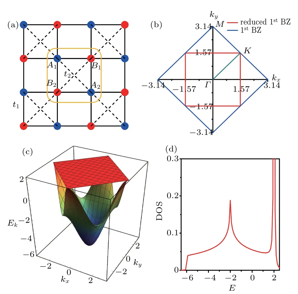
Fig.1.(a)The checkerboard lattice.The blue(red)dots represent lattice sites of the A(B)sublattice. Black solid and black dashed lines represent nearest-neighbor and diagonal links,respectively.We choose the distance between the nearest neighbors as the length unit in this article. The yellow box containing four lattice sites marks one cluster used in the CDMFT calculation.(b)The first Brillouin zone(BZ)of the checkerboard lattice.We also show the reduced first Brillouin zone for the chosen cluster in CDMFT calculations.High-symmetry points of the BZ are marked with Γ,K,and M.(c)Non-interacting band structure of a tight-binding model on a homogeneous(t2=t1)checkerboard lattice.(d)Non-interacting density of states when t2=t1.

2.Model and method

We consider the standard Hubbard model on the anisotropic checkerboard lattice at half filling.Its Hamiltonian can be written as

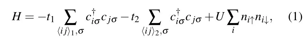
To start with,we first look at the non-interacting(U=0)band structure,which is readily obtained by diagonalizing the kinetic-energy terms(the first two terms on the right hand side of Eq.(1)).The energy of the resulting two bands is

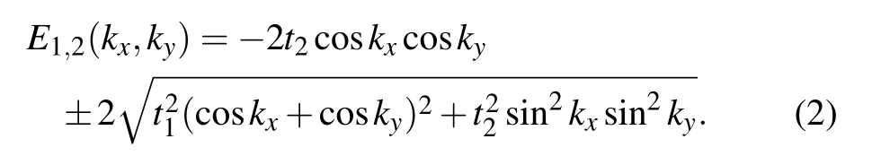
We plot the dispersions along high symmetry lines of the first Brillouin zone(see Fig.1(b))with different frustration strengths(t2)at half filling in Fig.2.When t2=0,there is no frustration and the lattice effectively reduces to a square lattice with perfect Fermi-surface nesting,which leads to a Mott insulating phase with any finite positive U at zero temperature.For the fully-frustrated case or isotropic case with t2=t1,the upper band becomes completely flat;the lower dispersive band touches it quadratically at the corner of the first Brillouin zone.We also plot the band structure over the whole first Brillouin zone and the corresponding density of states(DOS)of the homogeneous case(t1=t2)in Figs.1(c)and 1(d),respectively. At half-filling,the chemical potential sits at this band-touching point or right at the flat band,which causes divergences in perturbative calculations.[2,30–32]In this article,we take a numerical approach to this model,covering a wide range of frustration strength from the frustration-free case to the fully-frustrated one at finite temperatures.

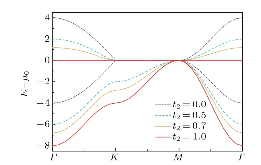
Fig.2. Non-interacting band dispersions along high symmetry lines(see Fig.1(b))with different frustration strengths at half filling. We choose t1=1 as the energy unit.µ0 is the chemical potential at half filling.

Our analysis of the interplay between geometrical frustration and electron–electron interaction in the half-filled checkerboard lattice is bases on the cellular dynamical meanfield theory(CDMFT)[33–35]calculation combined with continuous time quantum Monte Carlo method(CTQMC),[36,37]which has been widely applied to strongly correlated geometrically frustrated systems. The main idea of CDMFT is to map a system on a lattice to an impurity model by considering a cluster embedded in a self-consistent effective Weiss field. This impurity model is then solved using CTQMC,which updates the effective Weiss field and completes one self-consistent loop.Using this CDMFT approach,we calculate the single-particle Green’s function at imaginary frequencies,which is then analytically continued to real frequencies via the maximum entropy method.[38]With the single-particle Green’s function,one can further calculate physical quantities like DOS,magnetization,and spectral functions.

In our calculation,we choose four sites marked by a yellow circle as one cluster as shown in Fig.1(a),and the corresponding reduced first Brillouin zone is shown in Fig.1(b).We set t1=1 as the energy unit so that t2can be regarded as the frustration strength or the anisotropic parameter.Convergence is achieved by iterating the CDMFT self-consistent loop,and in each iteration 107QMC steps are performed.We work with the grand canonical ensemble and the half-filling condition is realized by adjusting the chemical potential.

3.CDMFT results

We focus on two important aspects of phase transitions in this system,metal–insulator transitions and magnetic transitions.The former is identified by looking at the DOS,where an energy gap at the chemical potential indicates an insulating phase,and vice versa. The latter is determined through the corresponding magnetic order parameter.

3.1.Metal–insulator transitions

For fixed frustration strength t2,the system goes through the typical Mott transition to a insulating phase when the interaction strength U is increased.This can be seen from Fig.3,where each subfigure corresponds to a fixed frustration and shows plots of DOS at different interaction strengths.

For example,figure 3(a)is the non-frustrated case with temperature T=0.05 and t2=0. One can see that when U is small,there is a Fermi-liquid-like peak near the Fermi energy,which is then split into a pseudogap structure when the interaction increases.[39,40]When the interaction strength is larger than a critical value,which is Uc=2.3 for this case,the DOS develops an obvious energy gap at the chemical potential,which indicates that the system undergoes a Mott transition from a metallic phase to a Mott insulating phase.Similarly,from Figs.3(b)and 3(c),one can read out Uc=2.8 and 4.3 for t2=0.2 and 0.5,respectively.We can see that the critical interaction strength of Mott transition increases with the frustration strength increasing. We also calculated the DOS with a higher temperature T=0.1 and t2=0.5 which is plotted in Fig.3(d)and shows Uc=4.9.It is consistent with the general picture that thermal fluctuations make it more difficult to drive a system to an ordered phase.

Fig.3.Density of states at different interaction strengths with(a)T=0.05,t2=0,(b)T=0.05,t2=0.2,(c)T=0.05,t2=0.5,and(d)T=0.1,t2=0.5.The frequency ω(which is also the energy,because we set the reduced Planck constant to unity)is counted from the chemical potential.

To gain a finer view of the Mott transition,it is instructive to look at the double occupancy(Docc)defined aswhere Nc=4 is the number of sites in one cluster.It indicates the average possibility of two particles occupying the same site.We calculated Doccas a function of U at different temperatures and frustration strengths,and the result is shown in Fig.4,where the arrows with different colors mark the corresponding phase transition points.It can be seen that Doccdecreases with an increasing interaction strength,which is a signature of Mott transition. In the large U limit in the Mott insulating phase,the system is almost singly occupied,i.e.,most particles are localized and hopping between lattice sites is forbidden by the strong on-site interactions.Moreover,when temperature is high(see plots with T=0.1 and 0.2 in Fig.4),Doccdecreases smoothly as U increases,indicating that the Mott transition is continuous.At lower temperature(see plots with T=0.05 in Fig.4),however,there is a visible discontinuity in Doccaround Uc. This suggests that the transition is a first-order transition at low temperatures.[9,28,41]

In addition,we further calculate the distribution of the spectral weight at the chemical potential with different interaction strength.It is a good characterization of interaction effects and can be directly accessed via angle resolved photoemission spectroscopy(ARPES)experiments.The result with T=0.05,t2=0.5 is shown in Fig.5.When U=3,smaller than the critical interaction strength Uc=4.3 for Mott transition,the spectral function has sharp peaks,indicating welldefined quasiparticles.Since it is calculated at zero frequency,it also shows a clear Fermi surface structure.[8]In the Mott insulating phase when U=6,sharp peaks disappear and no clear Fermi surface is shown.

Fig.4.Double occupancy as a function of the interaction strength U at different temperatures and frustration strengths.Arrows with different colors mark the corresponding positions of the critical U of the Mott transition.

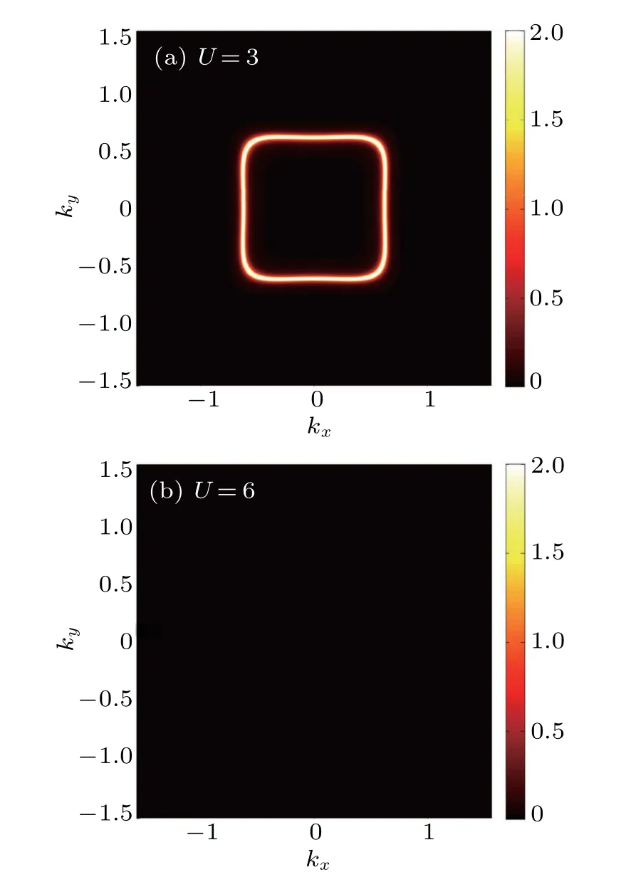
Fig.5.Distribution of the spectral weight at zero energy(the chemical potential)with(a)U=3 and(b)U=6.We choose T=0.05 and t2=0.5.For easy comparison,we use the same scale for spectral weight in these two plots.

3.2.Magnetic transitions

For magnetic transition, we focus on the antiferromagnetic order and define the order parameter as m=where sign(i)=−1(−1)if i belongs to sublattice A(B)(see Fig.1(a)). The calculation of m is straightforward with the single-particle Green’s function obtained.We plot m as a function of U at a fixed temperature and frustration strength(T=0.05,t2=0.7)together with the energy gap obtained from DOS under the same condition in Fig.6.When the interaction is weak,the magnetic order parameter is zero and the system is in a paramagnetic phase.At U=4.2,the system develops nonzero m with opposite signs between A and B sublattices,indicating an antiferromagnetic order.This is consistent with the fact that the strong interacting limit can be described by an antiferromagnetic Heisenberg model with frustration induced by t2.

With the information of the energy gap,one can further see that the development of a nonzero energy gap and a nonzero antiferromagnetic order do not occur simultaneously when T=0.05,t2=0.7.This leads to three phases,the paramagnetic metal phase(PM)when U<4.2,the antiferromagnetic metal(AFM)phase when 4.25.1.

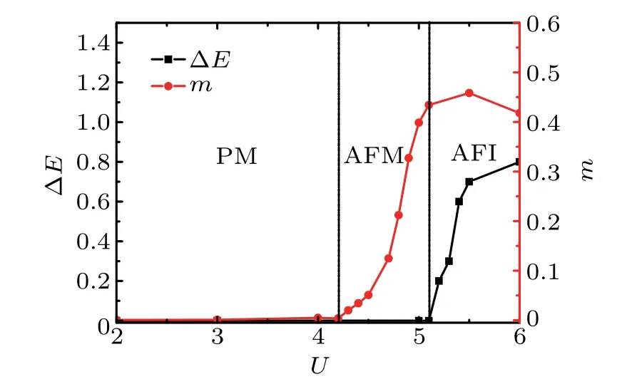
Fig.6.Antiferromagnetic order parameter m and single-particle energygap ∆E as a function of the interaction strength U when T=0.05 and t2=0.7.

3.3.Phase diagrams

Based on the above analysis of Mott transitions and magnetic transitions,we are ready to present phase diagrams which cover a wide area of the parameter space.

We first look at the result near zero temperature.Because zero temperature is not accessible through CTQMC,we approach the zero-temperature case by calculating at low temperatures,and a low-temperature(T=0.05)phase diagram in the t2–U plane is shown in Fig.7.It clearly shows the competing effect of magnetic frustrations and inter-particle interactions.An increasing interaction strength drives the system into an insulating phase with an antiferromagnetic order,while frustrations favor a metallic phase and suppress the magnetic order.Furthermore,the critical t2where antiferromagnetic order disappears tends to saturate when U increases.This suggests that when the frustration exceeds a critical value(here at t2≈0.9),it completely destroys the anti-ferromagnetic order even at the large U limit.This observation is consistent with previous studies that focus on the effect of frustration and deal with the Heisenberg model,[26]which effectively describes the large U limit of the model we considered here. The critical value of t2≈0.9 also agrees well with previous studies using different approaches.[30]In addition,there also exists a narrow window for an antiferromagnetic metal phase between the paramagnetic metal and antiferromagnetic insulator phases.

Fig.7.Phase diagram in the t2–U space with T=0.05.The red line is the phase boundary between the paramagnetic phase and the antiferromagnetic phase.The black line indicates the Mott transition(dashed line for first-order transitions and solid line for continuous ones).These two kinds of transitions divide the phase diagram to regions corresponding to paramagnetic metal(PM),antiferromagnetic metal(AFM),antiferromagnetic insulator(AFI),and paramagnetic insulator(PI)phases.The red star marks the critical point of the magnetic transition of the Heisenberg limit(U →∞)obtained by previous studies.[26]It can be seen that our calculation agrees with it well.

We also investigated the effect of thermal fluctuations by presenting a phase diagram on the T–U plane at a fixed frustration strength t2=0.5,as illustrated in Fig.8. One can see that thermal fluctuations and interparticle interactions also play competing roles in determining the phases of the system.As expected,when the temperature increases,the thermal fluctuations eventually destroy antiferromagnetic order as well as the Mott insulating phase and drive the system to a paramagnetic metal phase. During this transition,there is also an antiferromagnetic metallic phase in between.

Fig.8.Phase diagram in the T–U space at t2=0.5.

4.Discussion and summary

To summarize,we have studied Mott transitions and antiferromagnetic transitions on a half-filled anisotropic checkerboard lattice by means of the cellular dynamical mean field theory combined with the continuous-time quantum Monte Carlo method. We benchmark our calculation by looking at the critical frustration strength in the large-U limit,which can be effectively described by an antiferromagnetic Heisenberg model,and our result is consistent with previous studies.The interplay between frustrations(t2)(or anisotropy with the isotropic case being most frustrated),interparticle interactions(U),and thermal fluctuations(T)are investigated by varying the corresponding parameters.Through numerical simulations in a wide area of the parameter space,we extract phase diagrams of the system in the t2–U and T–U spaces. At fixed temperature and frustration strength,the interaction drives a Mott transition. When the interaction is sufficiently strong,the lattice sites are nearly singly occupied,and the system is in the insulating phase.This transition is accompanied by a magnetic transition,which tends to produce antiferromagnetic order when the interaction is strong.Thermal fluctuations and frustrations,on the other hand,play a competing role and favor metallic phases,and the magnetic order can be completely suppressed when t2and T exceed certain values.Besides,they further complicate the phase diagram by opening a narrow window for an antiferromagnetic metal phase.We hope that our study can provide useful information for future research on strongly-interacting systems on checkerboard lattices and related materials.

Acknowledgments

The author is grateful to G.Y.Cao,M.Huang,and S.J.Jiang for valuable comments and discussions. Numerical computations were partially carried out on a computer cluster of Wuhan Institute of Physics and Mathematics,Chinese Academy of Sciences.