Jiahui Hu(胡嘉卉), Jungang Wang(王俊刚), Yufeng Nie(聂玉峰),†, and Yanwei Luo(罗艳伟)

1Department of Applied Mathematics,Northwestern Polytechnical University,Xi’an 710129,China

2College of Science,Henan University of Technology,Zhengzhou 450001,China

Keywords:backward fractional Feynman–Kac equation,fractional substantial derivative,compact finite difference scheme,numerical inversion of Laplace transforms

1.Introduction

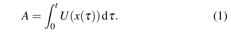
Diffusive motions exist widely in the nature,among the fields from condensed matter physics,[1–3]to hydrodynamics,[4]meteorology,[5]and finance.[6]Thus the Brownian functionals play important role in science community. Assume that x(t)is a path of a Brownian particle in the time interval(0,t),and U(x)is some prescribed function. Then a Brownian functional can be defined as.Since x(t)is a random path,A is a random variable. On account of the diversity of the function U(x),the Brownian functional A models various phenomena. In 1949,by using Feynman’s path integral method,Kac derived the(imaginary time)Schrödinger equation for the distribution function of A.[7]However,in recent years,by realizing that numerous anomalous diffusion phenomena exist widely in many systems,[8,9]the scientists pay more and more attention to the anomalous diffusion processes,or the non-Brownian motion,which can be modeled more exactly by fractional differential equations.[10]

Let x(t)be a trajectory of non-Brownian particle. The functional of anomalous diffusion has the same form as the Brownian functional

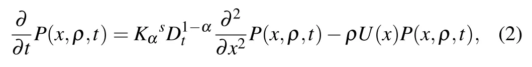
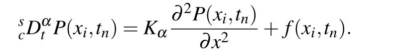
For the different prescribed function U(x),various physics processes can be characterized. For instance,when taking U(x)=1 in a given domain and to be zero otherwise,A models the time spent by a particle in the domain. The corresponding functional can be used in kinetic studies of chemical reactions that take place exclusively in the domain.[11,12]When the motion of the particles is non-Brownian in dispersive systems with inhomogeneous disorder,U(x)is given by x or x2.[12]By employing a versatile framework for describing the motion of particles in disordered systems,i.e.,the continuous time random walk(CTRW),derived the forward and backward fractional Feynman–Kac equations,[12–14]where the fractional substantial derivative is involved. The fractional substantial derivative is a time–space coupled operator,which is different from other fractional derivatives such as the Caputo and Riemann-Liouville types,and this newly proposed definition will be described in Definition 2.Both the forward and backward fractional Feynman–Kac equations describe the distributions of functionals of the widely observed subdiffusive processes.While in most cases scholars are only interested in the distribution of the functional A and regardless of the final position of the particle,it turns out to be more convenient to use the backward version.The backward fractional Feynman–Kac equation which is shown in Eq.(2),will be discussed detailedly in our work.Denote by P(x,A,t)the joint probability density function(PDF)of A and x at time t,which implies the process has started at x and the particle is found on A at time t. The backward fractional Feynman–Kac equation is given as[12–14]

For the past few years,numerical methods for solving fractional partial differential equations(PDEs)have been well developed,including finite difference methods,[16–20]finite element methods,[21–23]mixed finite element methods,[24,25]finite volume methods,[26,27]mixed finite volume element method,[28]and spectral methods,[29,30]etc. However,as for the PDEs with fractional substantial derivative involved,though there have been some literature for getting the numerical solutions(see Ref.[31]),high order finite difference schemes with the maximum norm error estimates have not been investigated yet.As is well known,high order schemes lead to more accurate results and less cost in computations if the solution of the equation is regular enough. Also,compared with the error estimates in discrete L2norm,the discrete L∞norm error estimates provide more immediate insight on the error occurring during time evolution.Thus,in practice,error estimates in the grid-independent maximum norm are preferred in numerical analysis. Noticing that the fractional substantial derivative is a non-local time–space coupled operator,it may bring more difficulty in constructing high order schemes for solving the corresponding equations,as well as in establishing the maximum norm error analysis.The purpose of this work is to develop efficient finite difference schemes for the backward fractional Feynman–Kac equation,which can achieve the q-th(q=1,2,3,4)order accuracy in temporal direction and the fourth order accuracy in spatial direction,respectively.The numerical stability and convergence in the maximum norm are discussed afterwards.Abundant numerical examples are also carried out to show the feasibility and the superiority of the proposed schemes.

The definitions of fractional substantial calculus are given as follows.[32]

Definition 1Let ν>0,ρ be a constant,and P(t)be piecewise continuous on(0,∞)and integrable on any finite subinterval of[0,∞).Then the fractional substantial integral of P(t)of order ν is defined as

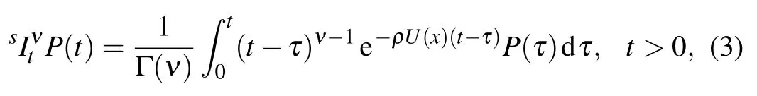
where U(x)is a prescribed function in Eq.(1).

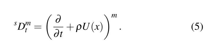
Definition 2Letµ>0,ρ be a constant,and P(t)be(m −1)-times continuously differentiable on(0,∞)and its m-times derivative be integrable on any finite subinterval of[0,∞),where m is the smallest integer that exceedsµ.Then the fractional substantial derivative of P(t)of orderµis defined as

where

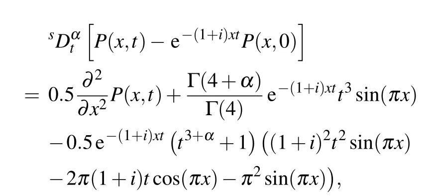
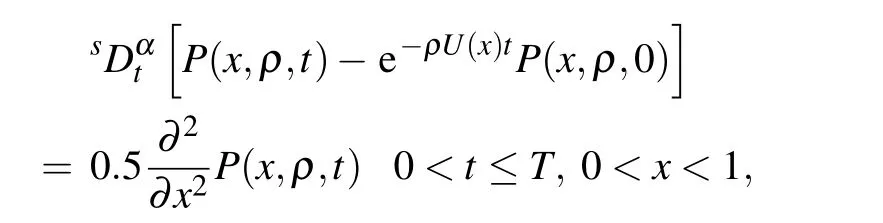
According to the definition of fractional substantial derivative,equation(2)can be expressed in the following form

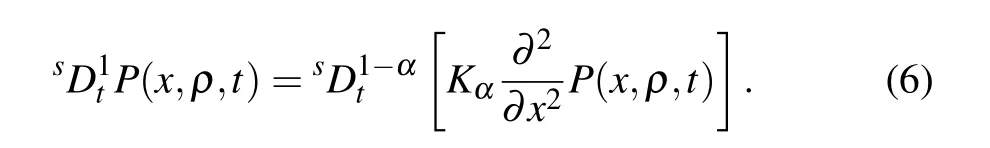
and then the equivalent form of Eq.(6)can be written as[31]

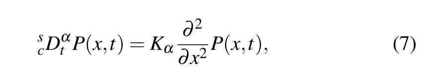
where P(x,ρ,t)is replaced by P(x,t)since ρ is given as a fixed constant.In the following two sections,we still use P(x,t)for convenience.

The remainder of this paper is organized as follows.In Section 2,for the backward fractional Feynman–Kac equation,the compact finite difference schemes with temporal q-th(q=1,2,3,4)order accuracy and spatial fourth order accuracy are established.In Section 3,by generalizing the inner product in Ref.[18]to complex space,we prove the unconditional stability and convergence of the first-order time discretization scheme in the maximum norm.In Section 4,extensive numerical examples are provided to verify the effectiveness and accuracy of the proposed schemes from the first to the fourth order time discretization.In particular,simulations of the backward fractional Feynman–Kac equation with Dirac delta function as the initial condition are carried out to further confirm the feasibility of the proposed methods. Finally we draw some conclusions in the last section.

2.Derivation of compact difference schemes

This section focuses on deriving compact difference schemes for the backward fractional Feynman–Kac equation,which are of the q-th(q=1,2,3,4)order approximation in temporal direction and the fourth order approximation in spatial direction,respectively.

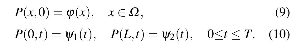
Without loss of generality,consider the backward fractional Feynman–Kac equation with a non-homogeneous source term in the interval Ω=(0,L),

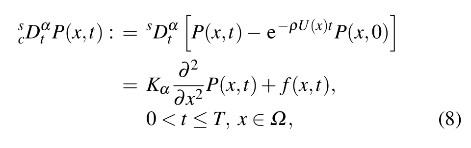
and the initial and boundary conditions are given as

Let M and N be two positive integers,then h=L/M and τ=T/N are the uniform size of spatial grid and time step,respectively.A spatial and temporal partition can be defined as xi=ih for i=0,1,...,M,and tn=nτ for n=0,1,...,N.Denote Ωh={xi|0 ≤i ≤M}and Ωτ={tn|0 ≤n ≤N}.Takeas the grid function space on Ωh.Then for any grid function,we have the following notations

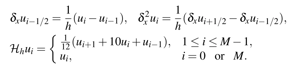
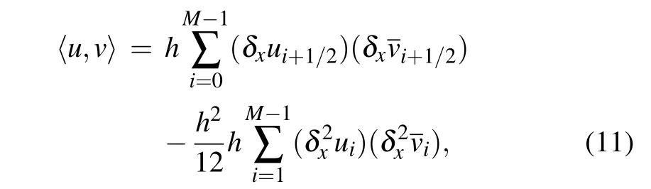
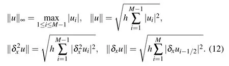
which can be verified directly according to the definition of inner product.Also,some norms which are necessary for the numerical analysis are shown below

For the inner product(11)and above norms,we have the following lemmas.

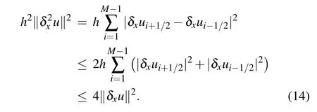
Lemma 1Forwe have

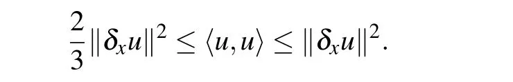
ProofFrom Eqs.(11)and(12),we obtain

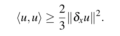
On the other hand,we have

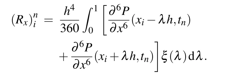
Lemma 3(Lemma 4.1 in Ref.[34])Let function g(x)∈C6[a,b]and ξ(λ)=5(1−λ)3−3(1−λ)5.Then

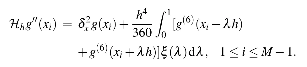
This completes the proof.

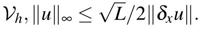
Lemma 2(Inequality(8.4.1)in Ref.[33])For ∀u ∈

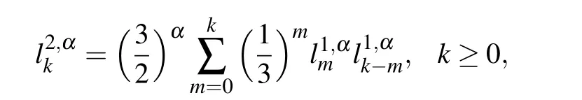
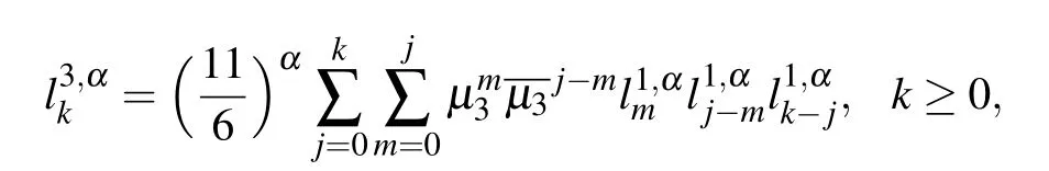
According to Ref.[32],the fractional substantial derivatives appeared in Eq.(8)have q-th order approximations,i.e.,

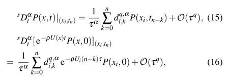
where

and

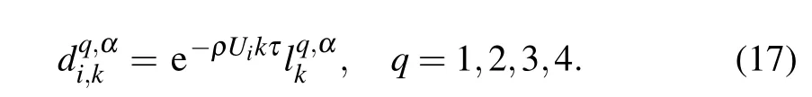
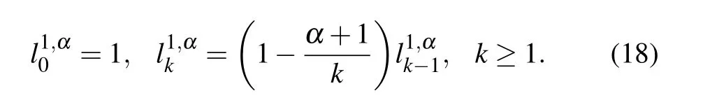
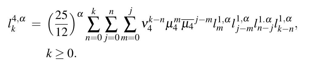
and

Denote

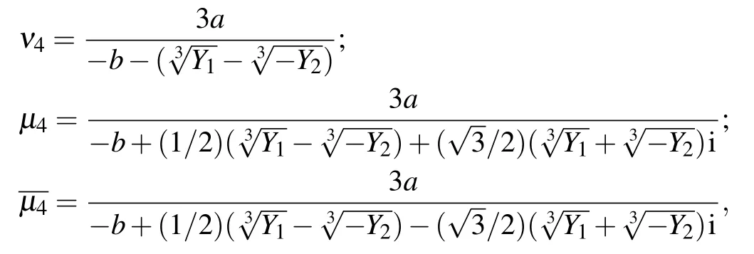
where a=−3/25,b=13/25,c=−23/25,d=1;A=b2−3ac,B=bc −9ad,C=c2−3bd;∆=B2−4AC>0,Y1=Ab+(3/2)a(−B −)>0,Y2=Ab+(3/2)a(−B+<0,then

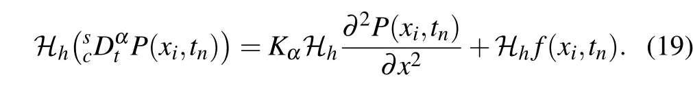
Considering Eq.(8)at the point(xi,tn),it can be written as

Acting the compact operatoron both sides of the above equation,we have

Therefore there exists a constantsuch that

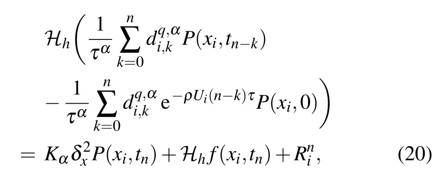
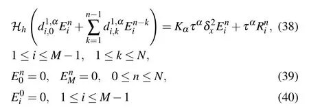
To execute the procedure,we rewrite Eq.(22)as the following equivalent form

It is necessary to point out that when n=1,the second term on the right-hand side of Eq.(25)vanishes automatically.

3.Stability and convergence analysis

In this section,we do the detailed theoretical analysis for the first order discretization in temporal direction of schemes(22)–(24).Letting U(x)=ω be a nonnegative constant,we introduce the properties of(k ≥0)first,and then prove the schemes are unconditionally stable and convergent in the maximum norm.

Lemma 4[31]The coefficientsdefined by Eq.(18)satisfy

and

Theorem 1The finite difference schemes(22)–(24)are unconditionally stable with the assumption(ρ)ω ≥0.

ProofAssumeis the approximate solution ofwhich is the exact solution of schemes(22)–(24),andis the approximation to ϕ(xi).Let0 ≤i ≤M,0 ≤n ≤N.From Eqs.(22)–(24),we have the perturbation error equations

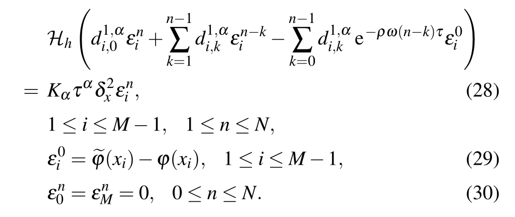
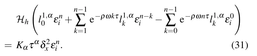
By use of Eq.(17),equation(28)can also be written as

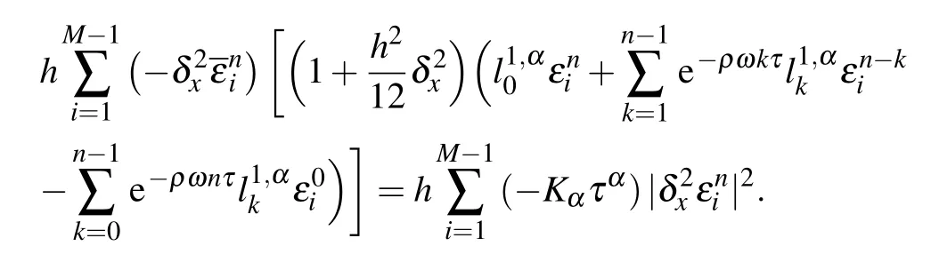
Using the summation formula by parts and noticing Eq.(30),we obtain

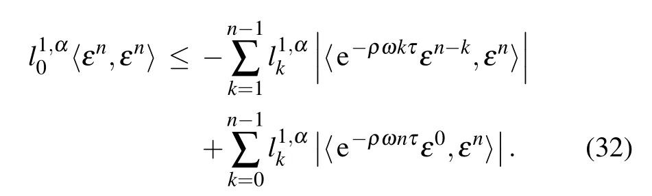
Then it can be deduced that the following inequality holds

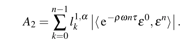
Let

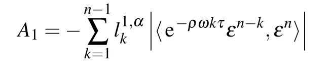
and

From the Cauchy–Schwarz inequality and Lemma 4,we have the estimates

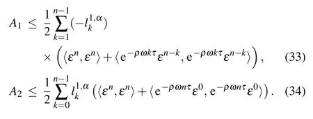
Combining inequalities(32),(33),and(34)with the assumptionω ≥0,it yields that

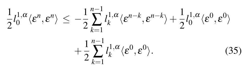
Next,we prove

by mathematical induction.In the case n=1,inequality(36)holds according to inequality(35). Suppose that for s=1,2,...,n−1,

holds.When s=n,according to inequalities(35)and(37),we have

Combining inequality(36)with Lemma 1 and Lemma 2,we conclude that

which completes the proof.

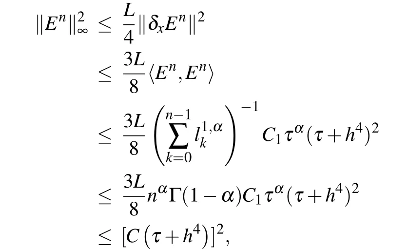
Theorem 2Letbe the solution of the finite difference schemes(22)–(24),and P(xi,tn)be the solution of the problems(8)–(10)with the assumption(ρ)ω ≥0.Denoting,0 ≤i ≤M,0 ≤n ≤N,then there exists a positive constant C such that

ProofAccording to Eqs.(20)and(22)–(24),we get the error equations

From Eq.(17),equation(41)can also be written as

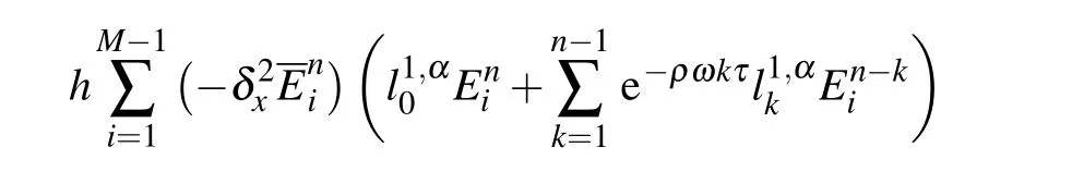
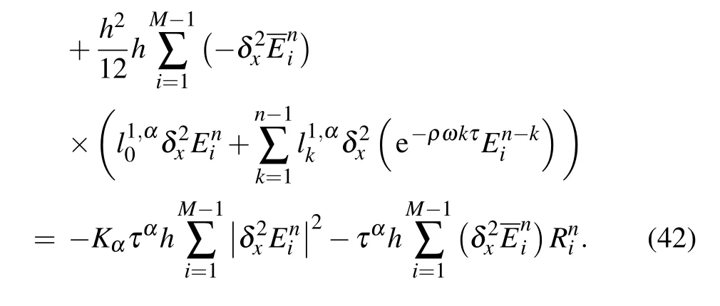
Using the summation formula by parts, we obtain from Eq.(42)

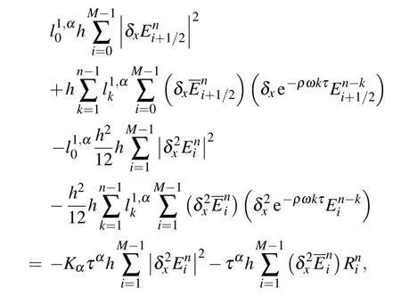
which implies

Then it can be deduced that

with the Cauchy-Schwarz inequality being used.

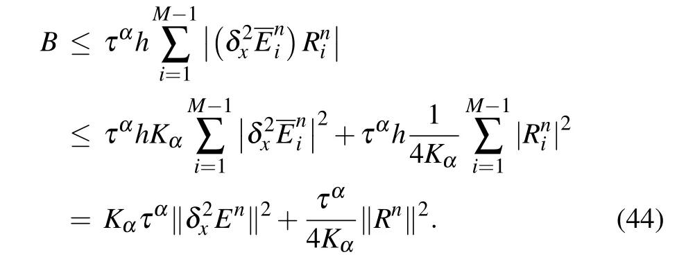
Let

It is observed that

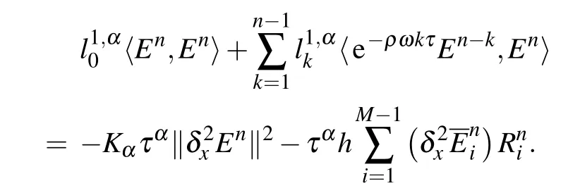
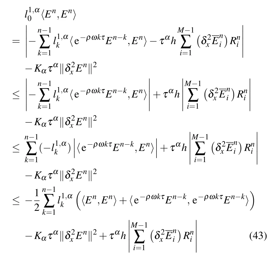
Substituting expression(44)into expression(43),and noticing inequality(45)with the assumption(ρ)ω ≥0,we have

and then it is derived from inequality(46)that

In the following,we prove

by mathematical induction.

For n=1,inequality(48)holds by inequality(47).Suppose

Then for s=n,by using inequalities(47)and(49)we conclude that

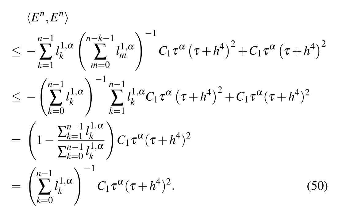
Finally,according to inequalities(50),(27),Lemma 1 and Lemma 2,we derive

4.Numerical examples

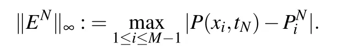
In this section,firstly we test some numerical examples to demonstrate the effectiveness of the schemes(22)–(24),and verify the theoretical results including convergence orders and numerical stability.The numerical errors is computed in the maximum norm,i.e.,

Then the backward fractional Feynman–Kac equation with Dirac delta function as the initial condition is simulated.By making use of the algorithm of numerical inversion of Laplace transforms,[36]we obtain the joint PDF P(x,A,t),and then the marginal PDFs of A and x,respectively.In particular,the case U(x)=0 is considered,when equation(8)reduces to the fractional Fokker–Planck equation.[37–40]Comparing its solution with the marginal PDF of x,it is further confirmed the reliability of our numerical methods.

4.1.Numerical results for P(x,t)with ρ being a constant

In the following two examples,we choose U(x)=1 and x,respectively.

Example 1Consider

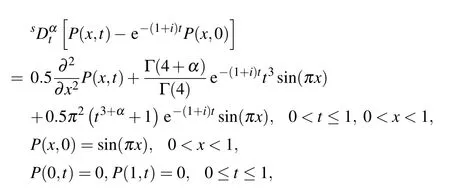
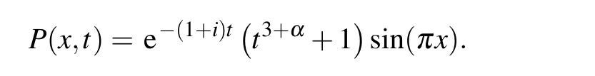
whose exact solution is known and is given by

In Table 1,an optimal step size ratio in temporal and spatial directions is adopted for Example 1 with q=1.As h and τ vary,the errors and convergence orders are reported in the table,which implies that the convergence orders in temporal and spatial directions are about one and four,respectively.It is in good agreement with the theoretical analysis.

Table 2 displays the computational results with an optimal step size ratio in temporal and spatial directions for Example 1 with q=2.It can be concluded from this table that the convergence orders with respect to time and space are approximately two and four,respectively.It agrees well with the theoretical results.

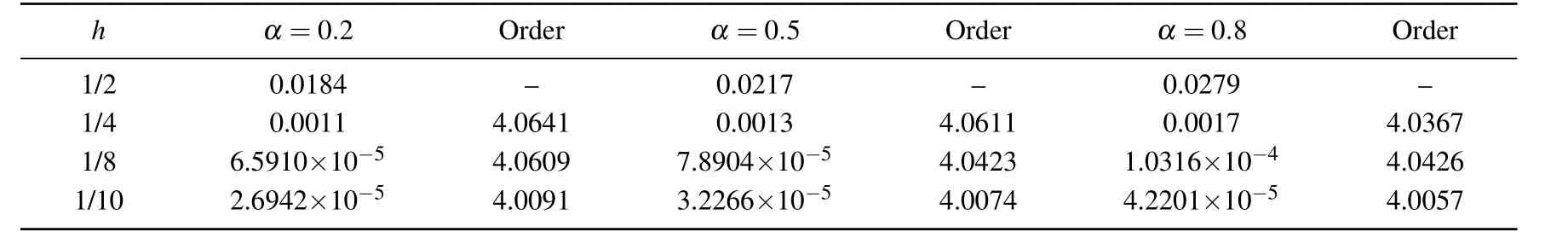
Table 1.The maximum errors and convergence orders with q=1 and an optimal step size ratio τ=h4(Example 1).

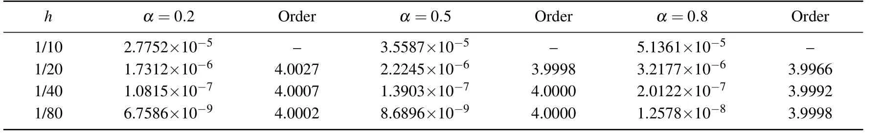
Table 2.The maximum errors and convergence orders with q=2 and an optimal step size ratio τ=h2(Example 1).

Example 2We now consider

whose exact solution is known and is given by

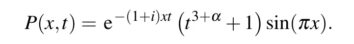
Table 3 shows the numerical errors and convergence orders in temporal direction for Example 2 with q=3.Let the step size h be fixed and small enough such that the dominating error arises from the approximation of the time derivative.Varying the step size in time,the numerical results are listed in this table,which is in accord with the theoretical analysis.

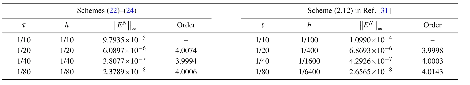
Tables 4–6 record the comparisons of schemes(22)–(24)with the scheme(2.12)in Ref.[31]for Example 2 with q=4.Taking an optimal step size ratio in temporal and spatial directions,these results report the convergence orders of schemes(22)–(24)with respect to time and space are both about four,which confirms the theoretical results.It also can be seen that even on the more coarse mesh schemes(22)–(24)get the smaller errors.These numerical results show that our method is not only reliable but also more efficient.

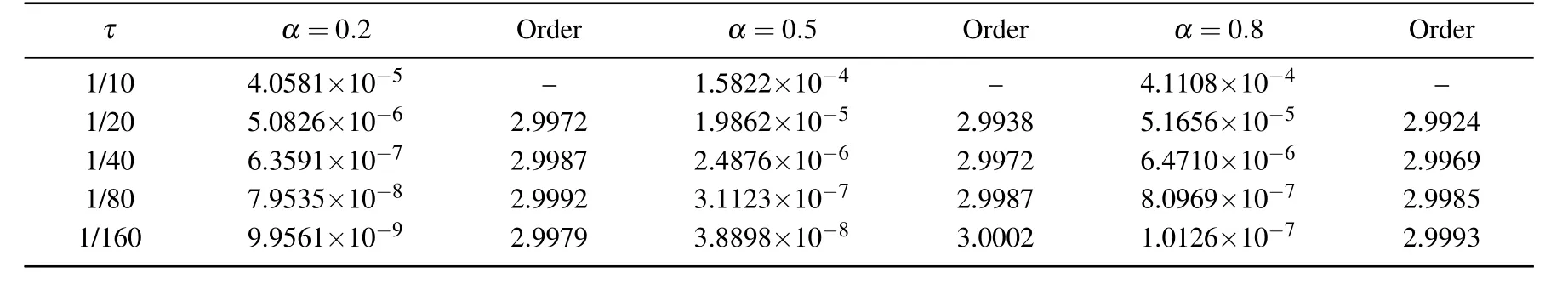
Table 3.The maximum errors and convergence orders in temporal direction with q=3 and h=1/1000(Example 2).

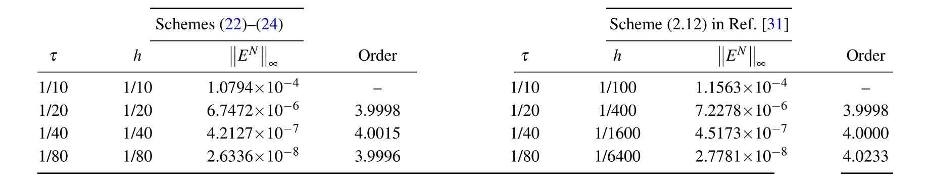
Table 4.Comparisons of errors and convergence orders obtained by schemes(22)–(24)and scheme(2.12)in Ref.[31]with α=0.1,q=4 and an optimal step size ratio for τ and h(Example 2).

Graphs of the modulus of errors for Example 2 with q=4 and α=0.4 are plotted in Fig.1.From these figures,we can find intuitively that,as the step sizes h and τ are reduced,the maximum of the modulus of the errors decreases gradually and approaches zero,which manifests the convergence of the presented algorithms.

4.2.Simulations with Dirac delta function as the initial condition

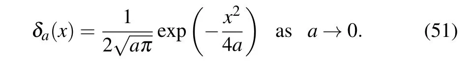
In this subsection,the backward fractional Feynman–Kac equation(8)with a zero forcing function and Dirac delta function as the initial condition is simulated.The Dirac delta function is defined by the limit of the sequence of Gaussians

For numerically getting the joint PDF P(x,A,t),the notation P(x,ρ,t)is reused instead of P(x,t).

Example 3Consider

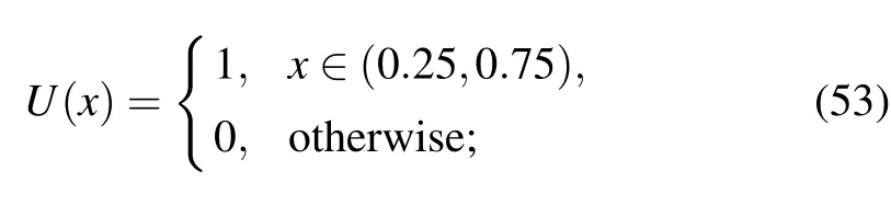
where U(x)is taken as

or

or

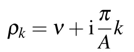
Suppose the joint PDF P(x,A,t)is a real function of A with P(x,A,t)=0 for A<0.The Laplace transform and its inversion formula are defined as

where ν>0 is arbitrary,but is greater than the real parts of all the singularities of P(x,ρ,t).

Fig.1.Evolution of the modulus of errors with q=4,α=0.4,and four different step sizes(Example 2).

Then the two marginal PDFs

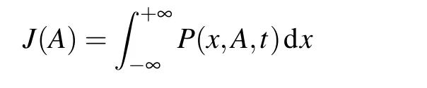
and

are derived by the composite trapezoidal formula.

For generating Figs.2–5,the procedure can be executed as follows.

Step 1For each fixed α,A,and ρk(k=0,1,...,35),by employing schemes(22)–(24)with q=4,τ=h=1/200,we getat time T.

Step 2According to the numerical method,[36]we obtain P(x,A,t).

Step 3By making use of the composite trapezoidal formula,we get the marginal PDF J(A).

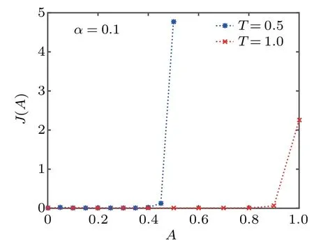
Fig.2.J(A)for Eq.(22)with U(x)defined in Eq.(52).

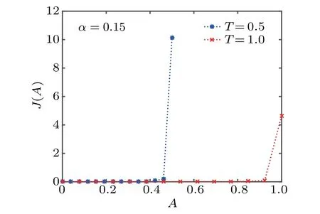
Fig.3.J(A)for Eq.(22)with U(x)defined in Eq.(53).

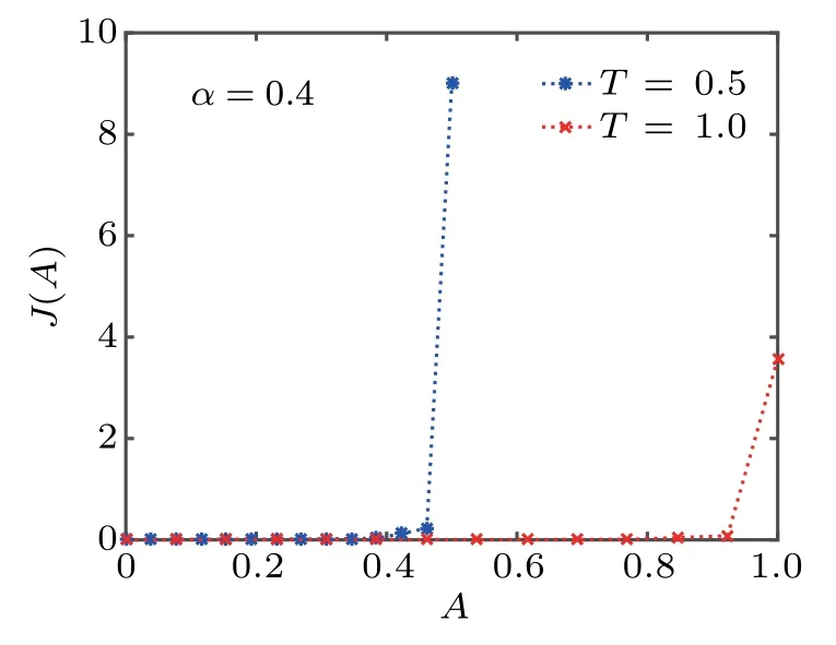
Fig.4.J(A)for Eq.(22)with U(x)defined in Eq.(53).

Fig.5.J(A)for Eq.(22)with U(x)defnied in Eq.(53).

Figures 2–5 present the curves of the marginal PDF J(A),where we can see the areas under the curves at time T=0.5 and T=1.0 are almost the same.It implies the conservation of probability.

The procedure of generating Figs.6–8 can be executed as follows.

Step 1TakeU(x)as defined in Eq.(54).For each fixed α,A,and ρk(k=0,1,...,35),by employing schemes(22)–(24)with q=4,τ=h=1/200,we get P(x,ρk,t)at time T=0.2.

Step 2According to the numerical method,[36]we obtain P(x,A,t).

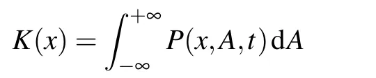
Step 3By making use of the composite trapezoidal formula,we have the marginal PDF K(x).

Step 4Letting U(x)=0 and using schemes(22)–(24)with q=4,we obtain the solution of the fractional Fokker–Planck equation KK(x).

Figures 6–8 depict the marginal PDF K(x),as well as the numerical solution of fractional Fokker–Planck equation KK(x).We can see K(x)coincides with KK(x),which further verified the effectiveness of the proposed schemes.

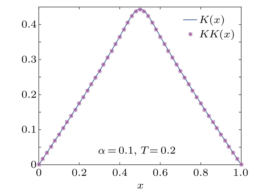
Fig.6.K(x)and KK(x)for Eq.(22),respectively.

Fig.7.K(x)and KK(x)for Eq.(22),respectively.

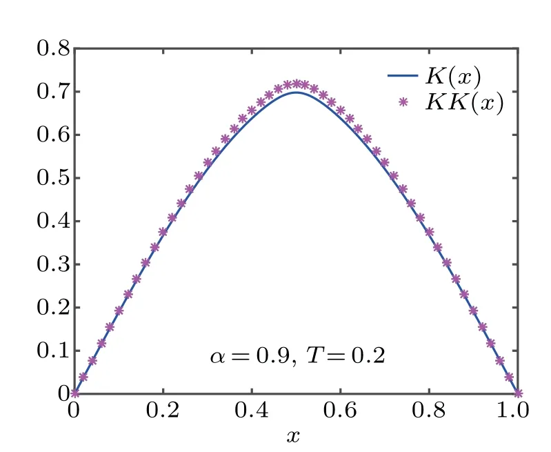
Fig.8.K(x)and KK(x)for Eq.(22),respectively.

5.Conclusion

In this paper,compact finite difference schemes for solving the backward fractional Feynman–Kac equation are proposed. These schemes are of the q-th(q=1,2,3,4)order accuracy in time and the fourth order accuracy in space,respectively.

By generalizing the inner product in Ref.[18]to complex space,we prove that the first-order time discretization scheme is unconditionally stable and convergent in maximum norm.For all the schemes proposed,from first to fourth order approximations in temporal direction,abundant numerical experiments are carried out to verify the theoretical analysis and their effectiveness.Moreover,the derived errors and convergence orders are compared with the corresponding results obtained in Ref.[31],which shows that the method in this work is more accurate and efficient. Also,the problem with Dirac delta function as the initial condition is simulated.By employing the algorithm of numerical inversion of Laplace transforms[36]and the composite trapezoidal formula,we draw the curves of the marginal PDFs,as well as the numerical solution of the fractional Fokker–Planck equation,which further confirm the effectiveness of our methods.