S. I. Onwukwe; N. C. Izuwa; E. E. Ileaboya; K. K. Ihekoronye

[a] Associate Professor, Federal University of Technology, Owerri, Nigeria.

[b]Senior Lecturer, Federal University of Technology, Owerri, Nigeria.

[c]Researcher, Federal University of Technology, Owerri, Nigeria.

Abstract Reviewing of some Niger Delta oil field reservoirs indicate that most of them are brown fields,thereby vulnerable to challenges such as; coning due to reduced size of the oil column, low oil production and lack of access to the residual oil trapped between existing wells of the brown field. Due to coning occurrences in the Niger-Delta brown oil field, most wells have been shut-in and a lot of recompletions are being made in order to combat this problem. To proffer solutions to these technical challenges of these brown oil fields, this study seeks to review the potentials of re-entry horizontal well technology and its viable application to optimizing oil production from brown oil field. Re-entry horizontal well Technology involves a method of converting an existing vertical well into an horizontal well to save cost as oppose to drilling a fresh horizontal well from the surface. The object of the re-entry well is to reduced cost,especially in areas where drilling costs are very high. The re-entry horizontal in this research was represented by a virtual horizontal well to study the potentials of producing brown fields.The simulation paradigm studied was Black oil with light oil type variation of 32O API. This article is therefore aimed at suggesting the conversion of existing vertical wells in the Niger-Delta into re-entry horizontal wells as a measure to optimize oil productionof these brown oil fields.

Key words: Brown fields; Conning; Reservoir simulation; Re-entry horizontal wells

1. INTRODUCTION

The term “brown field” has no single definition. Often, engineers consider fields brown when they have declined in production by more than 50% of their plateau rate. Different companies might apply their own specific definitions though. For example, Total Oil Company considers the surface and the subsurface in their definition. For the subsurface, they consider a field brown when the cumulative production has reached 50% of the initial 2P (proved and probable) reserves. And for the surface, they consider a field brown after 10 years of production. Halliburton Oil Company defines brown fields as fields where production has reached its peak and has started to decline.

Brown fields represent the backbone of global oil production and produce about two thirds of global daily average oil production and this percentage is increasing with time Syed (2012; 2009). Most of these brown fields were ones giant fields that have been produced over time, such that they are now acting like thin oil. And because these brown fields are now acting like thin oil, they are prone to all the challenges facing any thin oil.Understanding oil rim reservoir production dynamics is significant to successful development of these brown fields that have become thin oil rims. Thin oil rims development can be likened to the production of a large oil column towards the end of its economic life when abandonment would be strongly considered. Most Niger -Delta fields, for example the reservoir under consideration, are brown fields with vertical wells and as a result of production over time, are now thin oil reservoirs with thickness of about 40ft. These fields are still been produced by vertical wells where less oil and excess water are produced. Oil rim reservoirs are reservoirs that have small thickness from beginning, but thin oils vis-à-vis mature field are reservoirs that has been produced over time and whose thickness has become thin (small). This work intends to use the knowledge and application of oil rim reservoirs to handle a mature reservoir that has become thin oil by inputting some reservoir fluid and rock data into Eclipse (version, 2006), a commercial simulator, to model the existing reservoir and also to evaluate the before and after potentials of using re-entry horizontal wells vis-à-vis current vertical wells.Blaskovich (2000) affirmed that the world average of oil recovery factor is estimated to be 35% and that additional recovery over this “easy oil” depends on the availability of appropriate technologies with economic viability, and valuable reservoir management strategies. Javed (1995) stated that the discovery rate for the massive fields peaked in the late 1960s and early 1970s and declined outstandingly in the last two decades. The author further stated that about thirty massive fields comprise half of the world's oil reserves and most of them are categorized as brown field. Babadagli (2001) stated that the development of brown fields entails new and economically viable techniques, and proper reservoir management strategies.

2. LITERATURE REVIEW

A survey of literature shows that remarkable amount of research work has been done ranging from experimental studies to analytical and numerical simulation studies in order to know and predict water coning and cresting in vertical and horizontal wells respectively. Thin oil reserves despite their low pay thickness can still contain significant volumes of hydrocarbons-in-place. One important issue of thin oil column reservoirs is water and gas coning problems that have a negative effect on the ultimate oil recovery, and hence the project economics.Maximizing oil recovery of thin oil columns is a challenge because of coning of unwanted fluids, regardless of well orientation. Vo et al (1999) pointed out that oil and gas recovery from a thin oil column strongly depends on the oil column thickness, formation permeability, gas-cap size, aquifer strength, reservoir geometry, bed-dip magnitude, and oil viscosity. They further stated that the use of reservoir modeling to select a completion strategy (well placement, length, distance to fluid contacts, rate) and forecast performance are essential. Kabir et al (Kabir, Agamini, & Holguin, 2008, pp.73-82) stated that developing thin oil columns using horizontal wells improve hydrocarbon recovery from the reservoirs. They confirmed that it has been extensively used in recent years. Papatzacos et al (1989) stated that larger capacity to produce oil at the same drawdown and a longer breakthrough time at a given production rate as some of the advantages of using a horizontal well over a conventional vertical well. Joshi (2003) stated that horizontal wells have been used to produce thin zones,fractured reservoirs, formations with water and gas coning problems, waterflooding, heavy oil reservoirs, gas reservoirs, and in EOR method such as thermal and CO2 flooding. Joshi (Joshi, 1991) stated that the purpose of the horizontal wells was to enhance well productivity, reduce water and gas coning, intersect natural fractures and to improve well economics. Figure 1 below shows the placement technique of horizontal wells and also its large surface area contact with the hydrocarbon in the thin oil column.

Figure 1: Horizontal drilling / conventional drilling

Muskat and Wyckoff (1935, pp.114 &144) stated that coning result from the movement of reservoir fluids in the direction of least resistance, balanced by a tendency of the fluids to maintain gravity equilibrium. Onwukwe(2012, pp.1-10) noted that coning occurs when viscous forces exceed gravity forces near the wellbore of a producing well, which results in a high gas-oil ratio (GOR) in case of gas coning, or high water cut (BS&W) in case of water coning. The author further stated that water and gas coning are common in oil rim reservoirs, with attendant consequences of drastic drop in reservoir pressure and the overall recovery efficiency. Kimbrell (2001)stated that in thin oil column, the presence of oil-water contact hinders production of liquid hydrocarbon and often causes early abandonment of the afflicted well even when relatively thick pay column are found. Also when the reservoir is water driven, encroachment of water will eventually pose serious water coning problem.He further stated that in most field development plan, the breakthrough at the production wells is put off as long as possible by an optimal well placement and by carefully manipulating fluid withdrawal and circulation rates.

Paris et al (2008) stated that oil column size, gas cap volume size, permeability, aquifer strength and oil viscosity are some of the sub-surface factors affecting the recovery process of thin oil reservoir. They further stated that these entire factors play an vital role in determining the fluid flow dynamics and recovery factor.

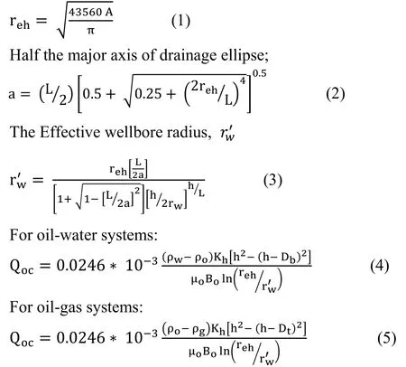
3. OIL CRITICAL FLOW RATE FOR WATER CONING

Loif et al (2012) defined Oil critical flow rate as the maximum rate at which oil is produced without production of water. Joshi (Joshi, 1988) derived the following relationships for determining the critical oil flow rate in horizontal wells by defining the following parameters.

The Horizontal well drainage radius reh

4. METHODOLOGY

The reservoir under consideration was a reservoir in the Niger-Delta, which has been in production over time and now behaving as thin oil. The reservoir was still been produced by vertical wells where less oil and excess water are produced. The challenge was how to extend the production life of this reservoir cost effectively by evaluating the before and after potentials of using re-entry horizontal wells vis-à-vis current vertical wells. To evaluate productivity index of the horizontal wells and to compare NPV Revenue and total cost of the horizontal well, as its conduit length increases. The structure map of the top of the reservoir was obtained from a field in Niger – Delta. This was then digitized for simulation purpose. Equations 4 and 5 of Joshi (Joshi, 1988) were used for calculating the critical oil flow rate in horizontal wells. The optimum well placement can be deduced graphically before used in the simulation.

4.1 Field Description

The reservoir was a simple, slightly elongated rollover anticline composed of a complex of coastal barrier sediments with predominantly fine grained, well-sorted micaceous sands. Figure 2 showed the structure map of the top of the reservoir. This reservoir was produced for a little above 40 year, the thickness of the pay zone was 40 ft. at a datum depth of 10120 ft. and overlain by a gas cap with an m-factor of 1.3. Table 1 showed the field data of the reservoir.

Figure 2: Structure map of the top of reservoir

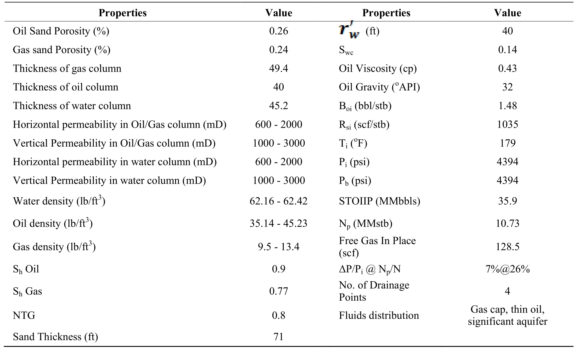
Table 1 Fluid and rock properties of reservoir

4.2 Reservoir Modelling and Simulation Using Eclipse

ECLIPSE was used to simulate production behavior of the reservoir with vertical wells and with re-entry horizontal wells. Schlumberger (2010) enlightened that ECLIPSE is an oil and gas reservoir simulator originally developed by Exploration Consultants Limited and currently owned, developed, marketed and maintained by Schlumberger. ECLIPSE uses the finite volume method to solve material and energy balance equations modeling. The reservoir covers an area of 37, 000ft by 25, 000ft and has a thickness of 40ft. A Horizontal well was drilled in the first layer at a depth of 10040 ft. and its length was changed considerably throughout the work from a minimum length of 200 ft. up to the length of 2000 ft. comprising of 10 different lengths. The reservoir model was used to guide the thin oil reservoir evaluation under four scenarios. The scenarios considered were:

a) The existing reservoir conditions was model as reference reservoir model,

b) The re-entry horizontal well was modeled into the scenarios, and

c) Single vertical, dual verticals and reentry horizontal well was then compared, and

d) Compare cumulative production as the horizontal well length was increased.

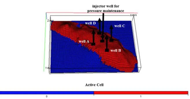
Figure 3: Eclipse illustration of full field active cells of the reservoir under study

Figure 4: Inverted 5–spot pattern simulation model

An inverted 5-Spot Pattern simulation model was used, having single injector well for pressure maintenance and four producer wells located in the corners of a square.

4.3 Results Presentation

After a simulation conversion of the vertical wells into re-entry horizontal wells, the simulation prediction of the wells was investigated and it was observed that wells were revived and oil production from the re-entry horizontal wells were increased considerably (see figures 5 to 12).

Figure 5: Well-a performance before re-entry work-over

Figure 6: Well-a performance after re-entry work-over

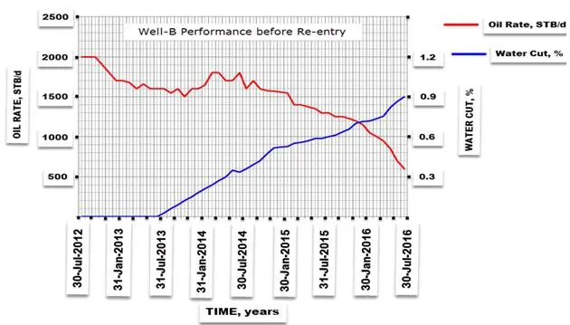
Figure 7: Well-B Performance before Re-entry work-over

Figure 8: Well-B Performance after Re-entry work-over

Figure 9: Well-c performance before re-entry work-over

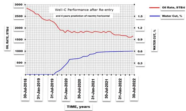
Figure 10: Well-c performance after re-entry work-over

Figure 11: Well-d performance before re-entry work-over

Figure 12: Well-d performance after re-entry work-over

4.4 DISCUSSION OF RESULT

From figure 5-6, well-A was completed in May, 1968 as a vertical producer with average net oil rate of 4,500 BOPD and zero water cut. The water production started in 1976 and increased rapidly with water cut of about 80% in 1996. Several work-over operations were carried out to shut off the water but failed because the water was coming quickly from the bottom as conning through the high vertical permeability.

The latest stability test conducted in July, 2015 showed an oil production rate of 1500 BOPD with about 60 %water cut, as shown in figure 5 (which illustrated a 5-year performance plot of Well-A before the re-entry horizontal). After a simulation conversion of the vertical Well-A to a horizontal well, the simulation prediction of the well was investigated and it was observed that Well-A was revived and oil production from the re-entry horizontal well was 3,500 BOPD of net oil and would drop to about 2,000 BOPD in 2022. Water cut was zero till 2019 and started to increase gradually until it reached about 33% at the end of prediction as shown in Figure 6.

From figure 7-8, well-B was completed in January, 1968 as a vertical producer with average net oil rate of 4,000 BOPD and zero water cut. The water production started also in 1976 and increased rapidly with water cut of about 80% in 1996. Also many work-over operations were carried out to shut off the water but failed because the water was coming quickly from the bottom as conning through the high vertical permeability.

The latest stability test conducted in July, 2015 showed an oil production rate of 1300 BOPD with about 60 %water cut, as shown in 7. After a simulation conversion of the vertical Well-B to a horizontal well, the simulation prediction of the well was investigated and it was observed that Well-B was revived and oil production from the re-entry horizontal well was 2,700 BOPD and would drop to about 1,700 BOPD in 2022.Water cut was 30% till 2019 and started to increase gradually until it reached about 60% at the end of prediction as shown in Figure 8.

From figure 9-10, well-C was completed in January, 1969 as a vertical producer with average net oil rate of 3,000 BOPD and zero water cut. The water production started in 1976 and increased rapidly with water cut of about 85% in 1996. Also just like wells A and B above, several work over operations were carried out to shut off the water but failed because the water was coming quickly from the bottom as coning through the high vertical permeability.

The latest stability test conducted in July, 2015 showed an oil production rate of 1300 BOPD with about 59 %water cut, as shown in figure 9. After a simulation conversion of the vertical Well-C to a horizontal well, the simulation prediction of the well was investigated and it was observed that Well-C was revived and oil production from the re-entry horizontal well was 2,800 BOPD of net oil and would drop to about 1,700 BOPD in 2022. Water cut was zero till 2019 and started to increase rapidly until reached about 60% at the end of prediction as shown in Figure 10.

From figure 11-12, well-D was completed in July, 1969 as a vertical producer with average net oil rate of 3,000 BOPD and zero water cut. The water production has started also in 1976 and increased rapidly with water cut of about 80% in 1996. Also just like wells A, B and C in the above, several work over operations were carried out to shut off the water but failed because the water was coning quickly from the bottom as coming through the high vertical permeability. The latest stability test conducted in July, 2015 showed an oil production rate of 1350 BOPD with about 80 % water cut, as shown in figure 11. After a simulation conversion of the vertical Well-D to a horizontal well, the simulation prediction of the well was investigated and it was observed that Well-D was revived and oil production from the re-entry horizontal well has started with net oil of 2,600 BOPD and would drop to about 1,600 BOPD in 2022. Water cut was 23% till 2019 and increased gradually to about 55% at the end of prediction as shown in Figure 12.

NOMENCLATURE

A =Drainage Area, acres.Bo =Oil formation volume factor, rb/stb.re =Drainage Radius, ft.reh =Horizontal Well Drainage Radius, ft.rw =Wellbore Radius, ft.rw′ =Effective Wellbore Radius, ft.A =Half the major axis of drainage ellipse, ft.L =Length of Horizontal Well, ft.Dt =Optimum distance from the top Db =Optimum distance from the bottomµo =Viscosity of Oil, cp.µw =Viscosity of Water, cp.ρg =Density of Gas, lb/ft3.ρo =Density of Oil, lb/ft3.ρw =Density of Water, lb/ft3.Kh =Horizontal Permeability, md.Qoc =Oil Critical Flow Rate.

CONCLUSIONS

Based on the research study conducted, following conclusions have been drawn:

a) Re-entry horizontal wells in mature oil fields have a promising potential.

b) Oil recovery is strongly dependent on the following sub-surface parameters, 1) thin oil thickness, 2) relative gas cap size (m-factor), 3) permeability, 4) oil viscosity, 5) aquifer strength. Thin oil development strategy needs to take into account and balance the effects of these factors.

c) Re-entry horizontal well technology is a proven technology.