WANG Yan-lin,XU Wei-man

(School of Mathematics and Statistics,Wuhan University,Wuhan 430072,China)

Abstract: In this paper,we investigate the smoothness effect for the Cauchy problem of Landau equation with γ ∈[0,1].Analytic estimate involving time and analytic smoothness effect of the solutions are established under some weak assumptions on the initial data.

Keywords: Landau equation;Boltzmann equation;analytic regularity;smoothness effect

1 Introduction and Main Results

In this paper,we study the Cauchy problem for the spatially homogeneous Landau equation,and investigate the analytic smoothing effect and moreover establish the explicit dependence on the time for the radius of analytic expansion. The Cauchy problem for spatially homogeneous Landau equation reads

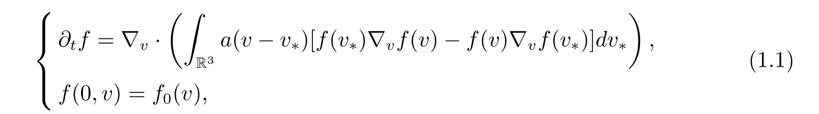
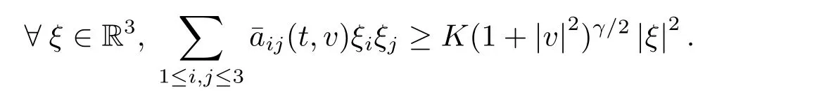
where f(t,v)≥0 stands for the density of particles with velocity v ∈R3at time t ≥0,and(aij)is a nonnegative symmetric matrix given by

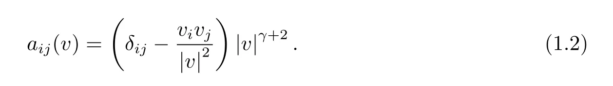
We only consider here the condition γ ∈[0,1],which is called the hard potential case when γ ∈(0,1]and the Maxwellian molecules case when γ=0.Set

and

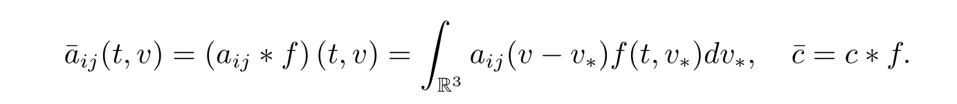
Then the Cauchy problem(1.1)can be rewritten as

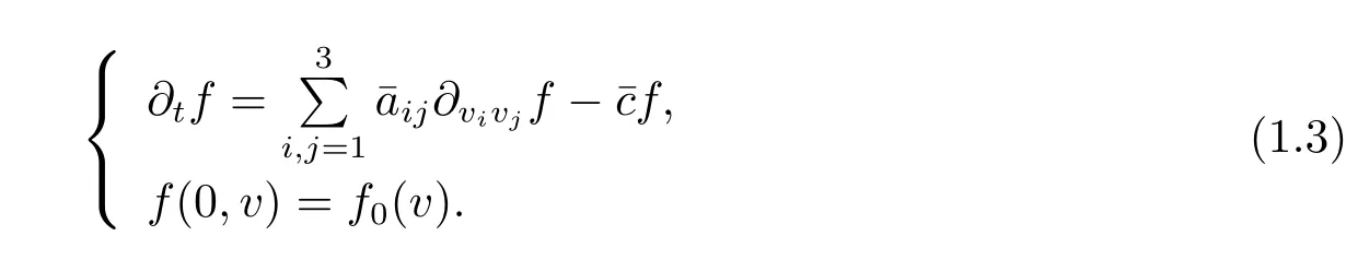
It is well-known that the Cauchy problem behaves similarly as heat equation,admitting smoothing effect due to the following intrinsic diffusion property of the Landau collision operator(c.f.[1,2])

There were extensive work to study the smoothing effect in different spaces.It was proved in[3]that when γ=0,the solutions to(1.3)enjoy ultra-analytic regularity for quite general initial data;that is statement of results in[13].

As far as the hard potential case is concerned,it seems natural to expect analytic regularity(see[5]),since the coefficients aijis only analytic function.This is different from the case γ=0,where the aijare polynomials and thus ultra-analytic.We mention that in[5]the dependence on the time t for the analytic radius is implicit.In this work we concentrate on the analysis of the explicit behavior as time varies. Our main result can be stated as follows.

Theorem 1.1Let f0be the initial datum with finite mass,energy and entropy and f(t,v)be any solution of the Cauchy problem(1.3). Then for all time t>0,f(t,v),as a real function of v variable,is analytic inMoreover,for all time t in the interval[0,T],where T is an arbitrary nonnegative constant,there exists a constant C,depending only on M0,E0,H0,γ and T such that for all

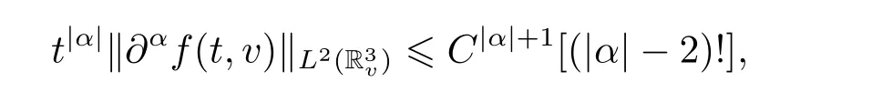
where α is an arbitrary multi-indices in N3.

The Landau equation can be obtained as a limit of the Boltzmann equation when the collisions become grazing,cf.[6]and references therein for more details.There were many results about the regularity of solutions for Boltzmann equation with singular cross sections and Landau equation(see[7–9])for the Sobolev smoothness results,and[10–13]for the Gevrey smoothness results for Boltzmann equation.And a lot of results were obtained on the Sobolev regularity and Gevrey regularity for the solutions of Landau equations,cf.[2,4,10,14–16]and references therein.In this paper,we mainly concern the analytic smoothness of the solutions for the spatially homogeneous Landau equation. Recently,Morimoto and Xu[3]proved the ultra-analytic effect for the Cauchy problem(1.3)for the Maxwellian molecules case,i.e.,f(t,·)∈A1/2(Rd).Chen,Li and Xu[5]proved the analytic smoothness effect for the solutions of Cauchy problem(1.3)in the potential case,which need a strict limit on the weak solutions of Cauchy problem(1.3),i.e.,with t0≥0 and C depending only on M0,E0,H0,γ and t0. Here we refer[5]and prove the analytic smoothness effect for the solutions of Cauchy problem(1.3)in the potential case without strict limit of solutions.And then we give a relatively better estimate form of f(t,v).

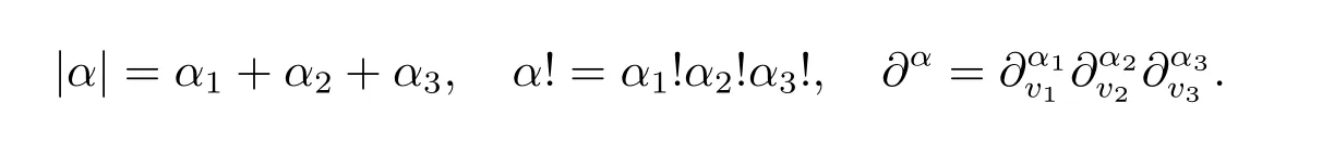
Now we give some notations in the paper.For a mult-index α=(α1,α2,α3),denote

We say β=(β1,β2,β3)≤(α1,α2,α3)=α if βi≤αifor each i.For a multi-index α and a nonnegative integer k with k ≤|α|,if no confusion occurs,we shall use α−k to denote some multi-indexsatisfyingandAs in[2],we denote by M(f(t)),E(f(t))and H(f(t))respectively the mass,energy and entropy of the function f(t,v),i.e.,

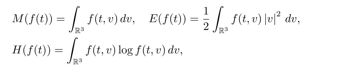
and denote M0=M(f(0)),E0=E(f(0))and H0=H(f(0)).It’s known that the solutions of the Landau equation satisfy the formal conservation laws

Here we adopt the following notations,

In the sequel,for simplicity of representation we always writeinstead of

Before stating our main theorem,we introduce the fact that in hard potential case,the existence,uniqueness and Sobolev regularity of the weak solution was studied by Desvillettes-Villani(see Theorems 5–7 of[2]).

We also state the definition of the analytic smoothness of f as follows.

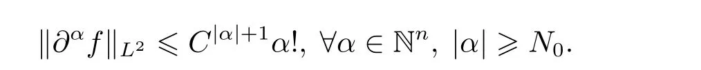
Definition 1.2f is called analytic function in Rn,if f ∈C∞(Rn),and there exists C>0,N0>0 such that

Starting from the smooth solution,we state our main result on the analytic regularity as follows.

Remark 1.3If f(t,v)in above still satisfies that for all time t0>0,and all integerwith c a constant depending only on M0,E0,H0,γ,m and t0.Then for all t>0,f(t,v),as a real function of v variable,is analytic in

Remark 1.4The result of Theorem 1.1 can be extended to any space dimensional case.

The arrangement of this paper is as follows:Section 2 is devoted to the proof of the main result. In Section 3,we present the proof of Proposition 2.3 in Section 2,which is crucial to the proof of main result here.

2 Proof of Main Result

This section is devoted to the proof of main result. To simplify the notations,in the following we always useto denote the summation over all the multi-indices β withandLikewisedenotes the summation over all the multi-indices β withandWe begin with the following lemma.

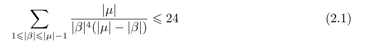
Lemma 2.1For all multi-indicesµ∈N3,we have

and

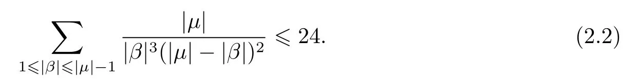
This lemma was proved in[5].

Next,we introduce the following crucial lemma,which is important in the proof of the Proposition 2.3. And the detailed proof of this lemma was given in[5]. Throughout the paper we always assume(−i)!=1 for nonnegative integer i.

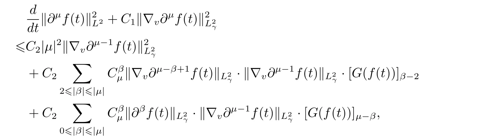
Lemma 2.2There exist positive constants B,C1,and C2>0 with B depending only on the dimension and C1,C2depending only on M0,E0,H0,and γ such that for all multi-indicesµ∈N3withand all t>0,we have

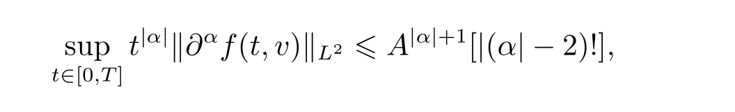
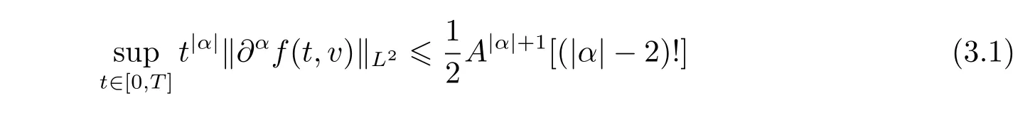
Proposition 2.3Let f0be the initial datum with finite mass,energy and entropy and f(t,v)be any solution of the Cauchy problem(1.3).Then for all t in the interval[0,T]with T being an arbitrary nonnegative constant,there exists a constant A,depending only on M0,E0,H0,γ,and T such that the following estimate holds for any multi-indices α ∈N3.

This proposition will be proved in Section 3.

Now we present the proof of the main result.

Proof of Theorem 1.1Given T0,for any multi-indices α,using estimate(2.3)in Proposition 2.3,there exists a constant A depending only on M0,E0,H0,γ,and T,such that

since

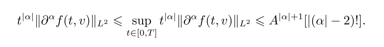
The proof of Theorem 1.1 is completed.

3 Proof of Proposition 2.3

This section is devoted to the proof of Proposition 2.3,which is important for the proof of the main result.

Proof of Proposition 2.3We use induction on|α|to prove estimate(2.3). First,when we take

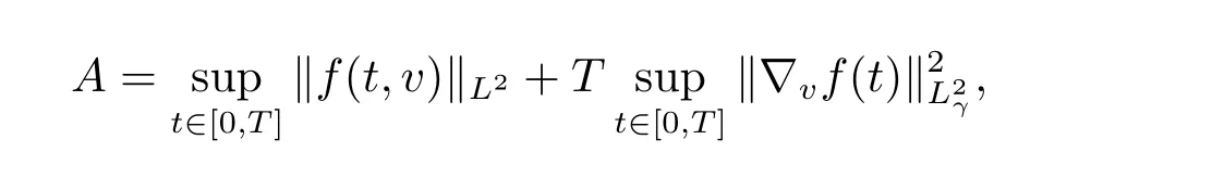
it is easy to find that estimate(2.3)is valid for|α|=0.

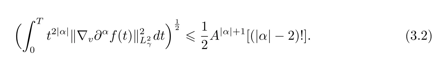
Now we assume estimate(2.3)holds for all|α|with,where integer k1.Next,we need to prove the validity of(2.3)for|α|=k,which is equivalent to show the following two estimates:for any|α|=k,

and

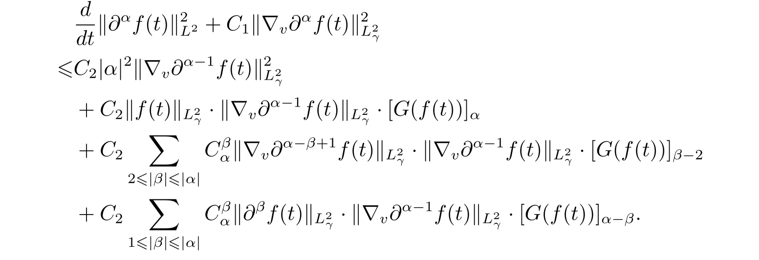
To begin with,we prove estimate(3.1). By means of Lemma 2.2 in Section 2,we obtain that

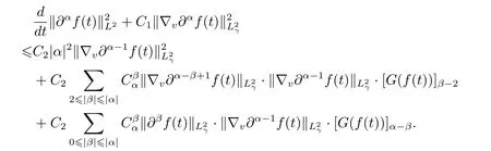
Rewriting the last term of the right-hand side of the inequality as

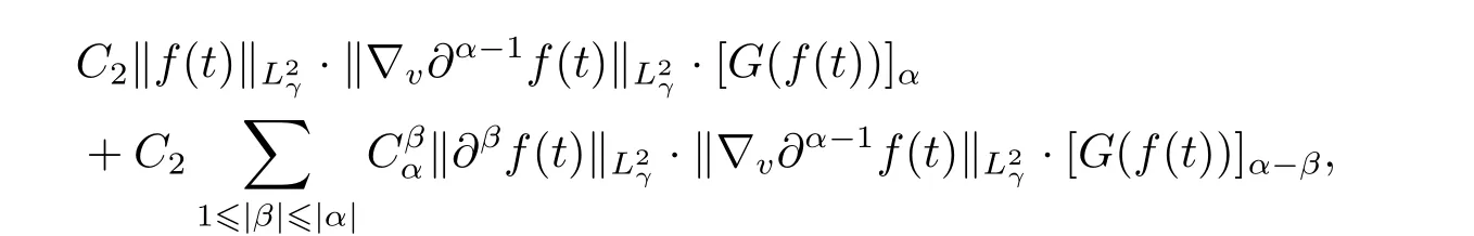
we get the following inequality

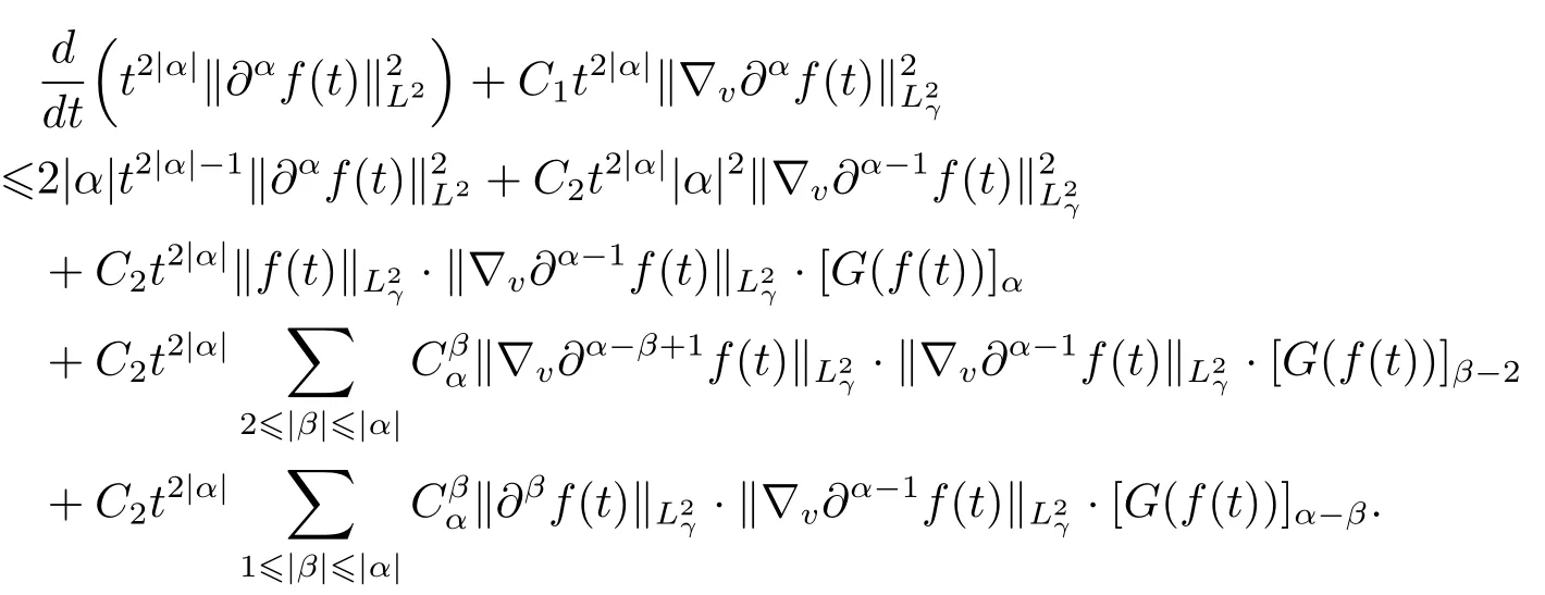
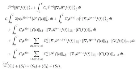
We multiply the term t2|α|in the both sides of the equality,leading to new inequality as follows

Integrating the inequality above with respect to t over the interval[0,T]to get that

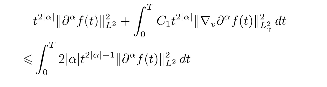
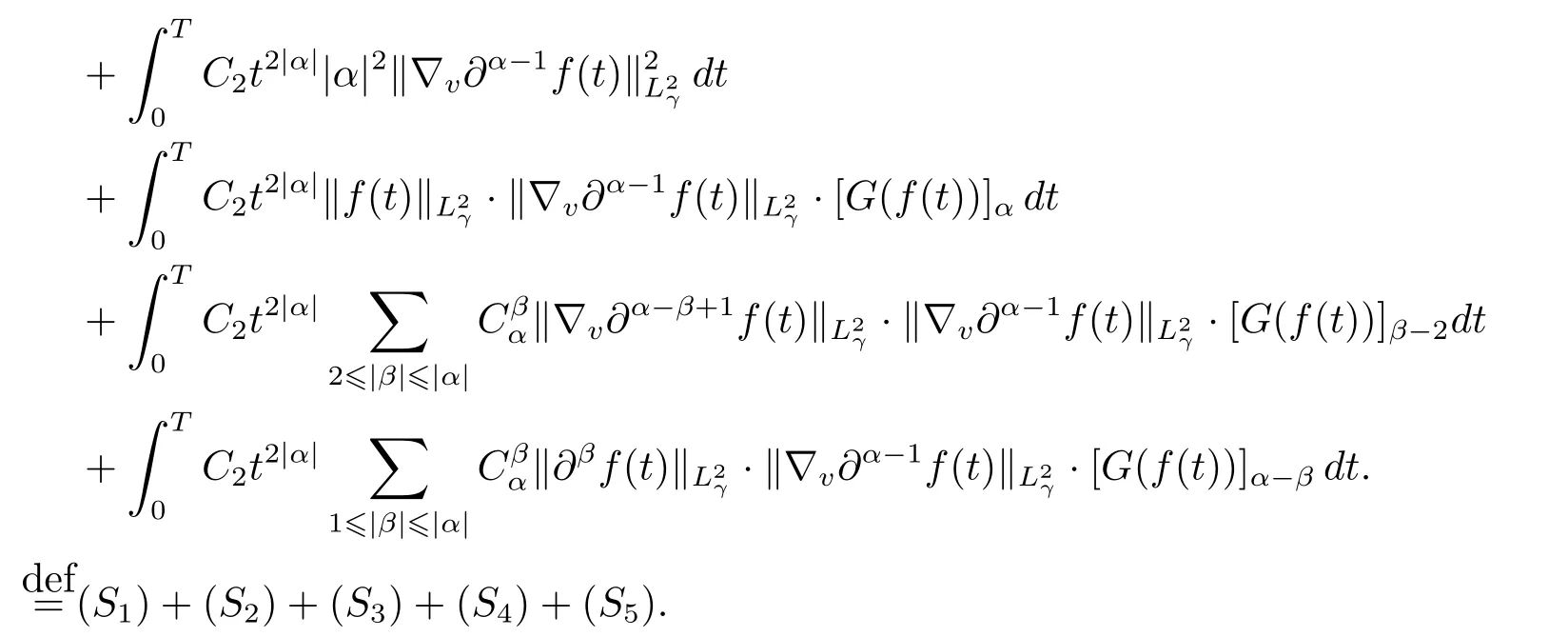
As a result,one has

since the fact that

To estimate these terms from(S1)to(S5)for all|α|=k,we need the following estimates which can be deduced directly from the induction hypothesis.The validity of(2.3)for allimplies that

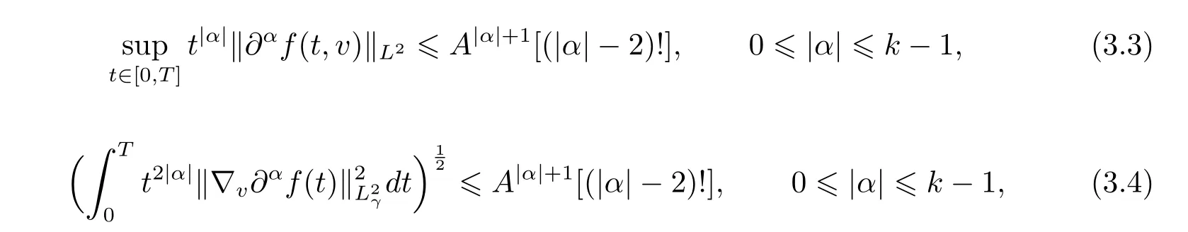
and

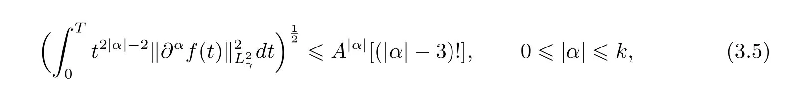
where A depends only on M0,E0,H0,γ and T.Inequality(3.5)follows from estimate(3.4),and the fact thatfor any multi-indices α withFor simplicity of presentation,we set

Consequently,if we take A large enough such that,then utilizing(3.3)–(3.6)with the factone has

and

That is,

where CTanddepends only on M0,E0,H0,γ and T.Now we are ready to treat terms(Sj)with|α|=k forIn the following process,we use the notationto denote different constants which are larger than 1 and depending only on M0,E0,H0,γ and T.Using the factand(3.5),we can show that

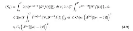
which is sound for all|α|=k.

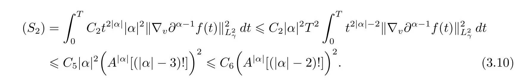
Next,by virtue of(3.4),one has

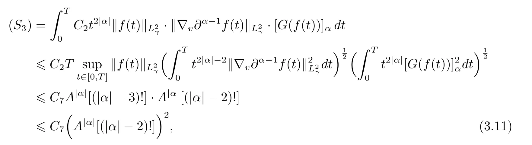
To estimate term(S3),by means of(3.4),(3.8)and Cauchy inequality,we obtain

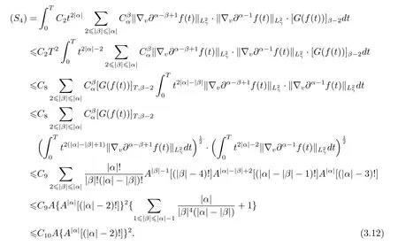
Now,we present the detailed estimate of term(S4),which makes full use of estimates(2.1),(3.4),(3.7),

Similarly,owing to estimates(2.2),(3.4),(3.5),(3.7),and Cauchy inequality,we obtain

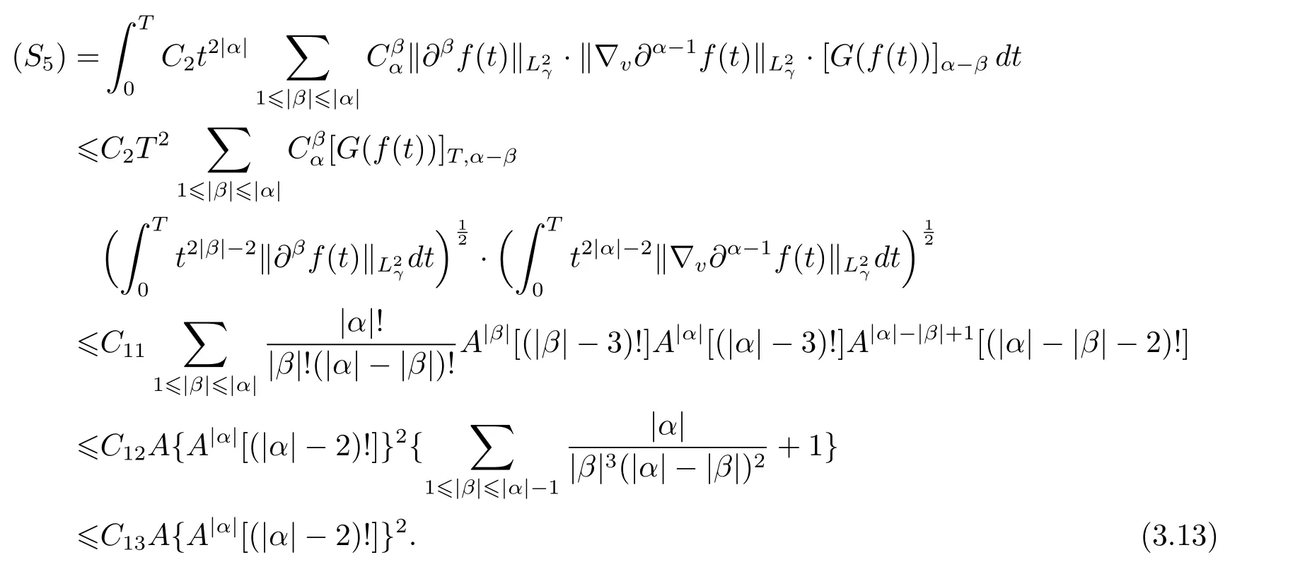
Consequently,it follows from the combining of estimates(3.9)–(3.13)that

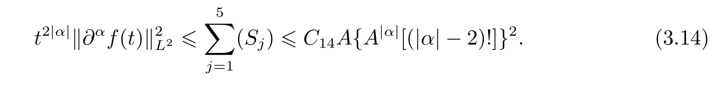
Taking A large enough such that

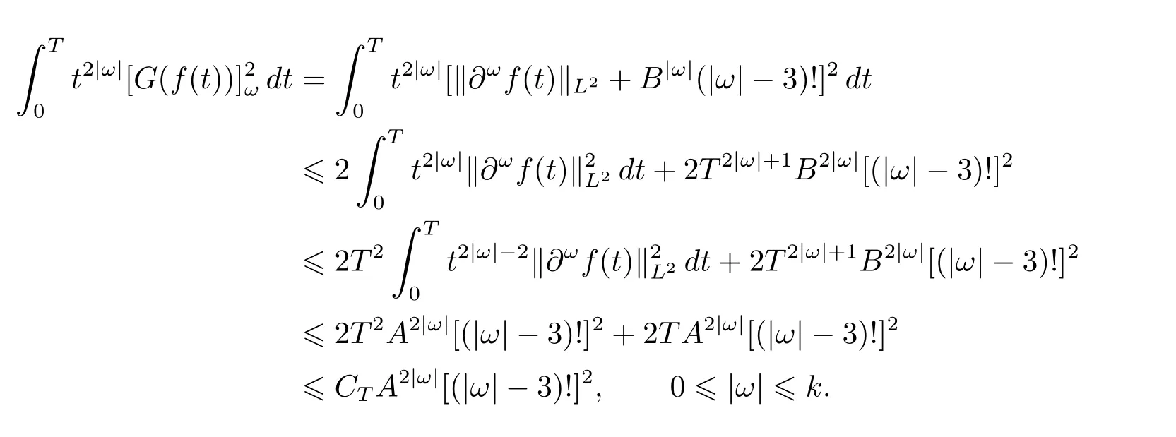
Now,it remains to prove estimate(3.2),for|α|=k,which can be handled similarly as the proof of estimate(3.1).Reviewing the process of the proof of estimate(3.1),we can find

Taking A as above,together with the fact that,we obtain

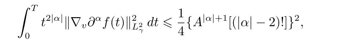
namely,estimate(3.2)is valid.The proof of Proposition 2.3 is completed.