Tengjin Zhao, Jing Zhang, Zhilin Li and Zhiyue Zhang,

Abstract: The validity of the tangent linear model (TLM) is studied numerically using the example of the Lorenz equations in this paper. The relationship between the limit of the validity time of the TLM and initial perturbations for the Lorenz equations is investigated using the Monte Carlo sampling method. A new error function between the nonlinear and the linear evolution of the perturbations is proposed. Furthermore, numerical sensitivity analysis is carried to establish the relationship between parameters and the validity of the TLM, such as the initial perturbation, the prediction time, the time step size and so on, by the method of mathematical statistics.

Keywords: Lorenz model, tangent linear model, nonlinear model, Monte Carlo.

1 Introduction

The study of chaotic systems has attracted a lot of attentions in the literature. The chaotic system in a population model is studied in depth by the Lorenz et al. [Lorenz (1963,1965, 1982); Yassen (2005); Wu, Xie, Fang et al. (2007); Zhao, Xing and Yu (2009)]. The chaotic system is characterized by a “sensitive dependence on initial condition” [Lorenz(1963)], such that the predictability of the future state is often severely limited by the chaotic dynamics of the system. The Lorenz model is one of the most popular models in dynamic systems, and has been studied by Wu et al. [Wu, Xie, Fang et al. (2007);Richter (2001); Yang, Chen and Yau (2002); Aniszewska and Rybaczuk (2005); Foias and Jolly (2005); Ding and Li (2012)]. In Shepelev et al. [Shepelev, Strelkova and Anishchenko(2018)], the transition from the regime of spatio-stationary structures and solitary states to complete incoherence in the network of nonlocally coupled Lorenz systems is numerically studied and a typical property of nonhyperbolic chaotic systems is obtained. Faghihnaini et al. [Faghihnaini and Shen (2018)] shows that the feedback loop produces periodic modes for three- and five-dimensional nondissipative Lorenz model. In Bougoffa et al. [Bougoffa,Al-Awfi and Bougouffa (2018)], the passage for Lorenz system to the third order non linear differential equation is established and for some special parameter values the obtained equation can be reduced to the well known equations.

The Lorenz model is the simplest model for dynamics of the convective layers and dynamics of closed convection loops.One application of the Lorenz model is the motion of a cell of fluid that is cooled from above and warmed from below.If the temperature difference between bottom and top is small,then the fluid of bottom will slowly rises because of the heating.If the temperature difference is large,then then he fluid from bottom may rise,and the colder fluid from button may drop at the same time[Lorenz(1963)].

The Lorenz model specifies a three-dimensional flow by the following non-dimensional equations:

where the parameters σ,r and b represent the Prandtl number,the Rayleigh number,and a geometric factor,respectively. The parameters have the values σ=10,r=28 and b=8/3,for which the well-known“butterfly”attractor exists.In Zhang et al.[Zhang,Mu,Zhou et al.(2017);Zhang,Liao and Zhang(2015)],the dynamical behavior of a generalized Lorenz system is derived based on the stability theory of dynamical systems so that the choice of parameters is reasonable.In addition,the state variables x,y,z represent measures of fluid velocity and the spatial temperature distribution in the fluid layer under gravity.The same sign x and y in the ODEs above indicates that the warm fluid is rising and the cold fluid is descending,which shows that a convection is taking place.

The linear approach assumes that the initial perturbation is sufficiently small such that its evolution can be governed approximately by the TLM instead of the nonlinear model.In the Lorenz model,the validity of the TLM depends on the initial perturbation,the time prediction,and the parameters in the model.However,there have been few papers addressing the numerical relationship between the parameters and the validity of the TLM.In the present study,the TLM is effective as long assatisfies a limited condition and we provide a confidence interval so that the validity can be described more precisely. Meanwhile we show the numerical relationship between parameters and the validity of the TLM,by the method of mathematical statistics.

Currently,there have been several predictability studies on the Lorenz model.The linear approach assumes that the initial perturbation is sufficiently small such that its evolution can be governed approximately by the TLM of the nonlinear model,and the computation of the linear fastest growing perturbation is reduced to the calculation of the linear singular vector and linear singular value.In order to study nonlinear mechanism of the amplification of the initial perturbations,Mu proposed the concept of the nonlinear singular vectors and nonlinear singular values. In Duan et al. [Duan and Mu(2009)],the concept of the conditional nonlinear optimal perturbation(CNOP)was introduced. The CNOP is the initial perturbation whose nonlinear evolution attains the maximal value of the cost function constructed according to the physical problems of interests at a specified time with physical constraint conditions and is called optimal.In Mu et al.[Mu and Zhang(2006)],the CNOP of a two-dimensional quasigeostrophic model is obtained numerically.In Wang et al.[Wang,Zhang and Zhu(2015)],the CNOP is applied to examine the non-linear and linear evolutions of perturbation in stochastic basic flows.The CNOP can be regarded as the most nonlinearly unstable initial perturbation superimposed on the basic state,which usually characterizes the structure of initial errors possessing the largest impact on the uncertainties at the prediction time. There exists a remarkable difference,if the initial perturbation becomes large,or the period is considerably long,or both.This means the TLM may fail to approximate the original nonlinear model.

Hence,we focus on the problem of the validity of the TLM by the Lorenz model.Compared with the TLM and the CNOP,a new objective function‖Mn(Φ0+φ0)-Mn(Φ0)-Ml(φ0)‖is introduced to combine the nonlinear mechanism of amplification of initial perturbations and the TLM of the nonlinear model.The relationship between several parameters and the validity of the TLM of the Lorenz model is studied by using the method of mathematical statistics.

The paper is organized as follows. In Section 2,the TLM of the Lorenz equations is introduced.In Sections 3 and 4,we analyze the effect of the parameters on the validity of the TLM for the Lorenz equations.In Section 5,the relationship between the limit of the time prediction of the validity of the TLM and the initial perturbation is established.Finally,some conclusions are given in Section 6.

2 TLM for the Lorenz equations

In this section,we first derive the TLM for the Lorenz equations. Adding perturbation(δx,δy,δz)to the state variables(x,y,z),we get

Using Eq.(1),we obtain the TLM for the Lorenz equations below if we omit the higher order terms δxδz and δxδy,

where(δx,δy,δz)is the perturbation of(x,y,z).

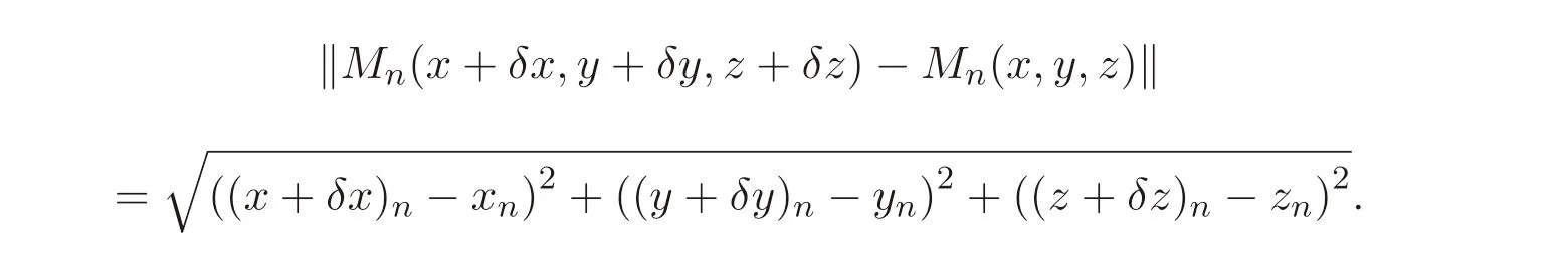
Corresponding to the definition of the TLM,the accuracy of program of the TLM is defined by the following formula:

where Mnrepresents the nonlinear model Eq.(1),Mlrepresents the TLM of MnEq.(3),and‖·‖denotes the L2norm,φ0is the perturbation of Φ0with 0 ＜α ＜1.In this paper,Φ0,φ0is the variable of vector of(x,y,z)and(δx,δy,δz).

Table 1:Results of the TLM program test

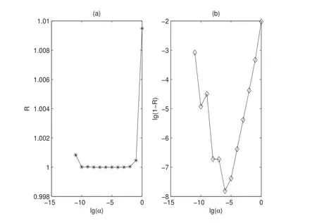
Figure 1:Results of the TLM program test

Tab.1 and Fig.1 all show that R consistently approximates to 1 as α approaches 0.It shows that the program of the TLM is correct and effective.By the way,the reason why α is so small that|R-1|gradually becomes large is the machine error which occurs for converting decimal digit to binary digit in computer.

3 The validity of the TLM

When the initial perturbation or the time prediction increases,the validity of the TLM may be destroyed[Farrell(1990)].In this study,we mainly consider the effect of r,T,Δt and the initial perturbation on the validity of the TLM,with σ=10 and b=8/3.

In this paper,we choose the Runge-Kutta discrete scheme[Verwer(1996);Guellal,Grimalt and Cherruault(1997);Zingg and Chisholm(1999)].Similarly,the last two equations are analyzed as the first equation:

where Pnrepresentsdenotesand Firepresents the ith equation of Eq.(1).

Combining Eq.(6)and Eq.(7),we obtain that

Expanding Eq.(8)by the Taylor formula,we get that

Similarly,we get that

In order to get the perturbation of the nonlinear evolution,making Qn((x+δx)n,(y+δy)n,(z+δz)n),then,we obtain that

Similarly,we obtain that

Then,the nonlinear evolution of perturbation can be described as

For the TLM,taking the similar discrete format,we obtain that

where LFidenotes the ith equation of Eq.(3),δPnrepresents(δxn,δyn,δzn)and δPn+1represents(δxn+1,δyn+1,δzn+1).

Similarly,we obtain that

Then,we can obtain the approximate error between nonlinear and linear evolution of perturbation:

Two kinds of initial state are chosen in numerical experiments. We set the parameters σ=10,b=8/3,r=28 and Time step Δt=0.01.

Experiment 1:the initial state is chosen as(-3.86,-8.77,21.2).

Fig.2 shows the evolution of error in the L2norm between nonlinear model and linear model.Therefore,the result of numerical experiment is close to theoretical analysis.In fact,not only the norm of approximating error,but also the components of state have the same result.In Fig.3,it is the evolution of δx,δy,δz,approximation between nonlinear and linear,respectively.

Figure 2:Evolution of the norm of the approximation error:(a)the result of numerical experiment,(b)the result of theoretical analysis

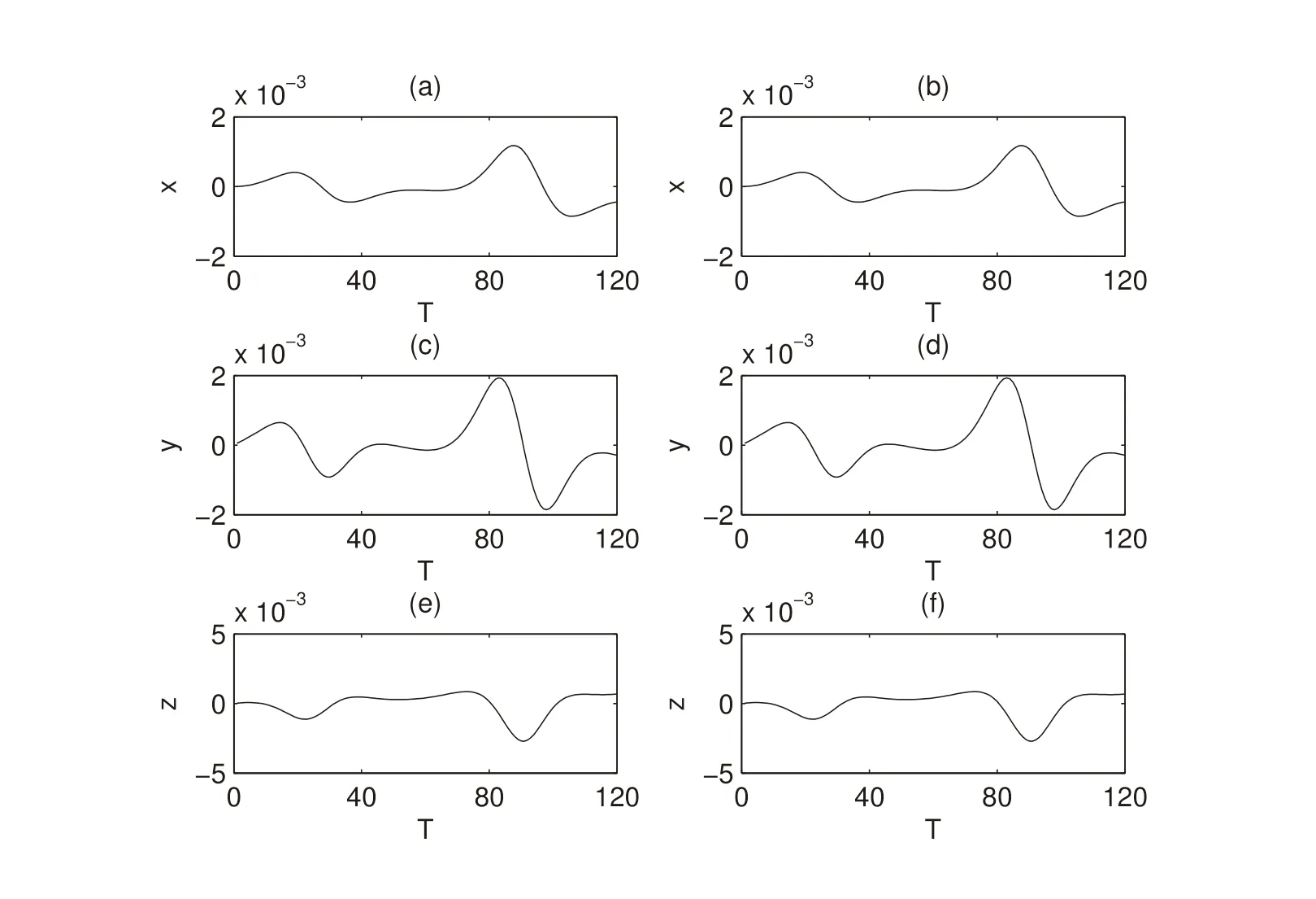
Figure 3:Evolution of each component of the approximation error:(a,c,e)the results of numerical experiment of δx,δy,δz,respectively;(b,d,f)the results of theoretical analysis of δx,δy,δz,respectively

Figure 4: Evolution of the norm of the approximation error when the initial state is:(a)the result of numerical experiment,(b)the result of theoretical analysis

The evolution of error in the L2norm between nonlinear model and linear model is depicted in Fig. 4 where(a)and(b)denote the result of numerical experiment and theoretical,respectively.The graphic of(a)is the same to the graphic of(b)so that the numerical scheme is effective.Fig.5 shows the evolution of δx,δy,δz,approximation between nonlinear and linear and also depicts the result of numerical experiment is close to theoretical analysis.

Figure 5: Evolution of the norm of the approximation error when the initial state is(a)the result of numerical experiment,(b)the result of theoretical analysis

4 The effect of parameters

The effect of parameters is studied in this section.Some scholars have studied the validity of the TLM by the evolutions of the CNOP or the linear singular vector,which needs two objective functions. Here,we use a new objective function to show the evolution.Furthermore,the validity of the TLM of the initial perturbation φ*is called the conditional nonlinear and linear optimal perturbation with constraint||φ0||≤σ and the objective function E(φ0),if and only if

We say that the TLM is valid as long as E(φ0)≤‖Φ0‖×η,for a given small number η.E(φ0)is the evolution error between the nonlinear and linear evolution and we denote it by E in the following.At the same time,we give a confidence interval if the parameter makes E satisfy‖Φ0‖×η ≤E(φ0)≤C‖Φ0‖×η for a constant C.The TLM is said to be valid if the parameters fall in the confidence interval.

As the initial state is(-3.86,-8.77,21.2),using the method of nonlinear least squares,we obtain that

Figure 6:The evolution error E for the initial state(-3.86,-8.77,21.2)in subgraphs(a,c,e)and the initial state in subgraphs(b,d,f);The evolution error E for r=1 in subgraphs(a,b),r=20 in subgraphs(c,d)and r=28 in subgraphs(e,f)

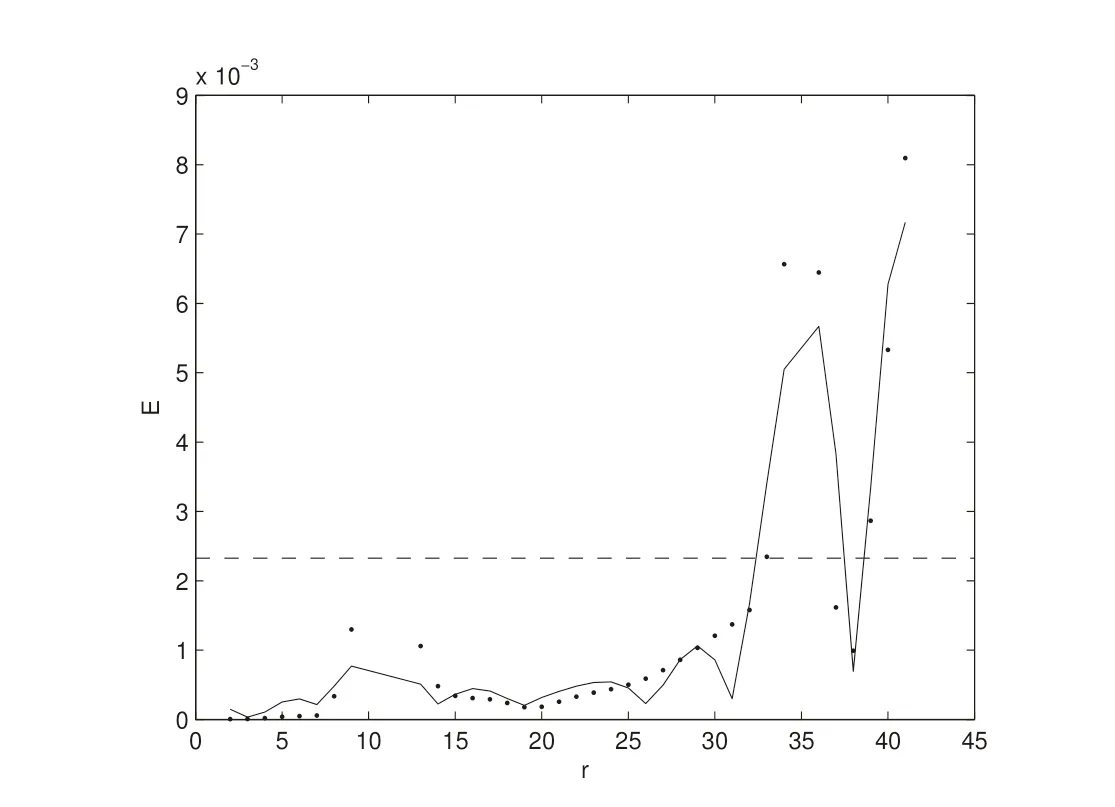
Figure 7: The dotted line denotes the scatter diagram of E and r and the full line denotes numerical simulation of the relationship between E and r for the initial state(-3.86,-8.77,21.2).The dash line denotes E=‖Φ0‖×10-4

Figure 8: The dotted line denotes the scatter diagram of E and r and the Full line denotes numerical simulation of the relationship between E and r for the initial stateThe dash line denotes E=‖Φ0‖×10-4

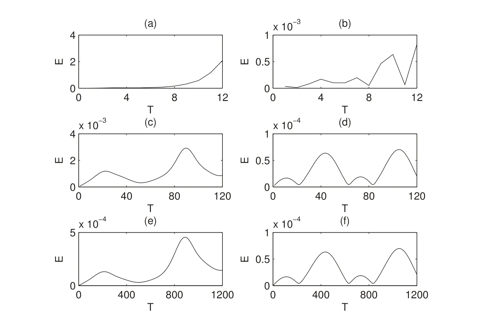
Figure 9:The evolution error E for the initial state(-3.86,-8.77,21.2)in subgraphs(a,c,e)and the initial state in subgraphs(b,d,f);The evolution error E for Δt=0.1 in subgraphs(a,b),Δt=0.01 in subgraphs(c,d)and Δt=0.001 in subgraphs(e,f)

As the initial state is(-3.86,-8.77,21.2),we get that

Figure 10: The dotted line denotes the scatter diagram of E and Δt and the full line denotes numerical simulation of the relationship between E and Δt for the initial state(-3.86,-8.77,21.2).The dash line and pecked line denote E=‖Φ0‖×10-4 and E=‖Φ0‖×10-3,respectively

In Fig.10,E ≤‖Φ0‖×10-4and the TLM is valid as Δt ≤0.025,for the initial state(-3.86,-8.77,21.2).Meanwhile,when E ≤‖Φ0‖×10-3,we can obtain that the TLM is valid whatever Δt is.[0.025,+∞)is the confidence interval.However,Fig.11 shows that Δt increases to 0.12,the TLM is valid for the initial stateWhen E ≤‖Φ0‖×10-4,Δt ≤0.14,the TLM is valid.Therefore,[0.12,0.14]is the confidence interval for the initial stateWe note that although the sample size is relatively small,the study is not affected.

Thirdly,the TLM is valid,when the initial perturbation is small enough in the pioneering work.There are little studies on the numerical relationship between the initial perturbation and the validity of the TLM.Let σ=10,b=8/3,r=28,T=120 and Δt=0.01.The initial perturbation is initial state times 0.1,0.01 and 0.001.

Figure 11: The dotted line denotes the scatter diagram of E and Δt and the full line denotes numerical simulation of the relationship between E and Δt for the initial stateThe dash line and pecked line denote E=‖Φ0‖×10-4 and E=‖Φ0‖×10-3,respectively

Figure 12:The evolution error E for the initial state(-3.86,-8.77,21.2)in subgraphs(a,c,e)and the initial state in subgraphs(b,d,f);The evolution error E for the initial perturbation 0.1 in subgraphs(a,b),the initial perturbation 0.01 in subgraphs(c,d)and the initial perturbation 0.001 in subgraphs(e,f)

As the initial state is(-3.86,-8.77,21.2)

Figure 13:The dotted line denotes the scatter diagram of E and the initial perturbation and the full line denotes numerical simulation of the relationship between E and the initial perturbation for the initial state(-3.86,-8.77,21.2).The dash line and pecked line denote E=‖Φ0‖×10-4 and E=‖Φ0‖×10-3,respectively

Fig.13 shows that the TLM is valid as‖φ0‖≤0.02 and E ≤‖Φ0‖×10-4.And the TLM is valid as‖φ0‖≤0.26 and E ≤‖Φ0‖×10-3.Therefore[0.02,0.26]is the confidence interval for the initial state(-3.86,-8.77,21.2).Similarly,we obtain that[0.3,0.86]is the confidence interval for the initial stateThe initial perturbation has obviously effect on the error of approximation between nonlinear and linear model.

Finally,let σ=-10,b=8/3,r=28,Δt=0.01,and initial perturbation is(x,y,z)times 0.01.We mainly analyze the effect of T,i.e.,T=120,T=500,T=1000.

Fig.15 shows that E becomes larger when T is larger.It means that the nonlinear evolution of the Lorenz model and the TLM is complicated and is hard to predict,as the terminal time T is large.And at the same time prediction,E is much smaller,when the initial state is close to the equilibrium point.

As the initial state is(-3.86,-8.77,21.2)

Figure 14:The dotted line denotes the scatter diagram of E and the initial perturbation and the full line denotes numerical simulation of the relationship between E and the initial perturbation for the initial state The dash line and pecked line denote E=‖Φ0‖×10-4 and E=‖Φ0‖×10-3,respectively

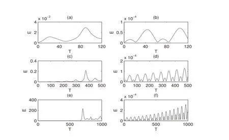
Figure 15:The evolution error E for the initial state(-3.86,-8.77,21.2)in subgraphs(a,c,e)and the initial statein subgraphs(b,d,f);The evolution error E for T=120 in subgraphs(a,b),T=500 in subgraphs(c,d)and T=1000 in subgraphs(e,f)

Figure 16: The dotted line denotes the scatter diagram of E and T and the full line denotes numerical simulation of the relationship between E and T for the initial stata(-3.86,-8.77,21.2). The dash line and pecked line denote E = ‖Φ0‖×10-4 and E=‖Φ0‖×10-3,respectively

Figure 17: The dotted line denotes the scatter diagram of E and T and the full line denotes numerical simulation of the relationship between E and T for the initial stata The dash line and pecked line denote E = ‖Φ0‖×10-4 and E=‖Φ0‖×10-3,respectively

From Fig.16 and Fig.17,E produces the periodic changing with T when T becomes small. It is the result of Lorenz model rather than an accidental phenomenon when the terminal time T is limited.In Fig.16,the TLM is valid when T ≤500.And the confidence interval can be omited since E=‖Φ0‖×10-3almost equals with E=‖Φ0‖×10-4and E is much greater as T increases. Similarly,T ≤2200,the TLM is valid,in Fig. 17.Whatever T is,the TLM is valid in the condition of E ≤‖Φ0‖×10-3.

5 Relationship between initial perturbation and the prediction time of validity of the TLM

The limit of the time prediction of validity of the TLM is defined as the time Tpat which‖Mn(Φ0+φ0)-Mn(Φ0)-Ml(φ0)‖≤‖Φ0‖×10-4.And Tpis the function of lg‖φ0‖.The parameters have the values σ=10,r=28,b=8/3,for which the well-known“butterfly”attractor exists.A long integration using the Runge-Kutta method with a time stepsize Δt=0.01 was performed to obtain 800 points within the attractor,with two kinds of initial states. A set of random errors,which have a Gaussian distribution with zero mean and the root-mean-square distance is magnitude‖φ0‖,were superimposed on the initial states to form an ensemble of perturbed states. An ensemble of 800 errors,which‖Mn(Φ0+φ0)-Mn(Φ0)-Ml(φ0)‖,at each time step was obtained by integrating solutions of the Lorenz model.The ensemble average of the magnitude of the errors was defined as the average error E.The ensemble average was taken as the geometric mean[Ding and Li(2012)].

Figure 18:Dotted line:scatter diagram of Tp and lg‖φ0‖;Full line:numerical simulation result of the relationship between Tp and lg‖φ0‖

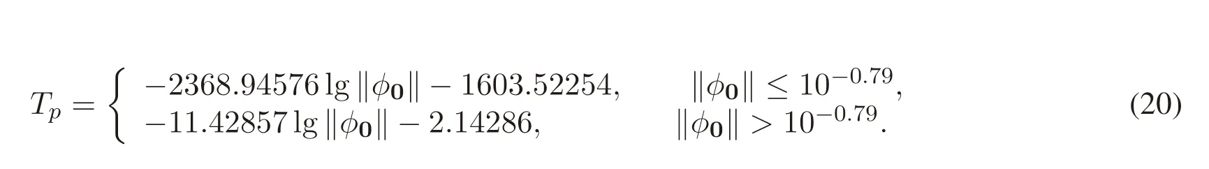
Fig.18 shows Tpas a function of lg‖φ0‖,with the initial state(-3.86,-8.77,21.2).Tpdecreases approximately linearly with increasing lg‖φ0‖for φ0≥10-2.6;however,Tpdecreases more quickly with increasing lg‖φ0‖for φ0≤10-2.6.Therefore,we conclude that the relationship between Tpand φ0in the Lorenz model can result from the logarithmic regression using Eq.(19).

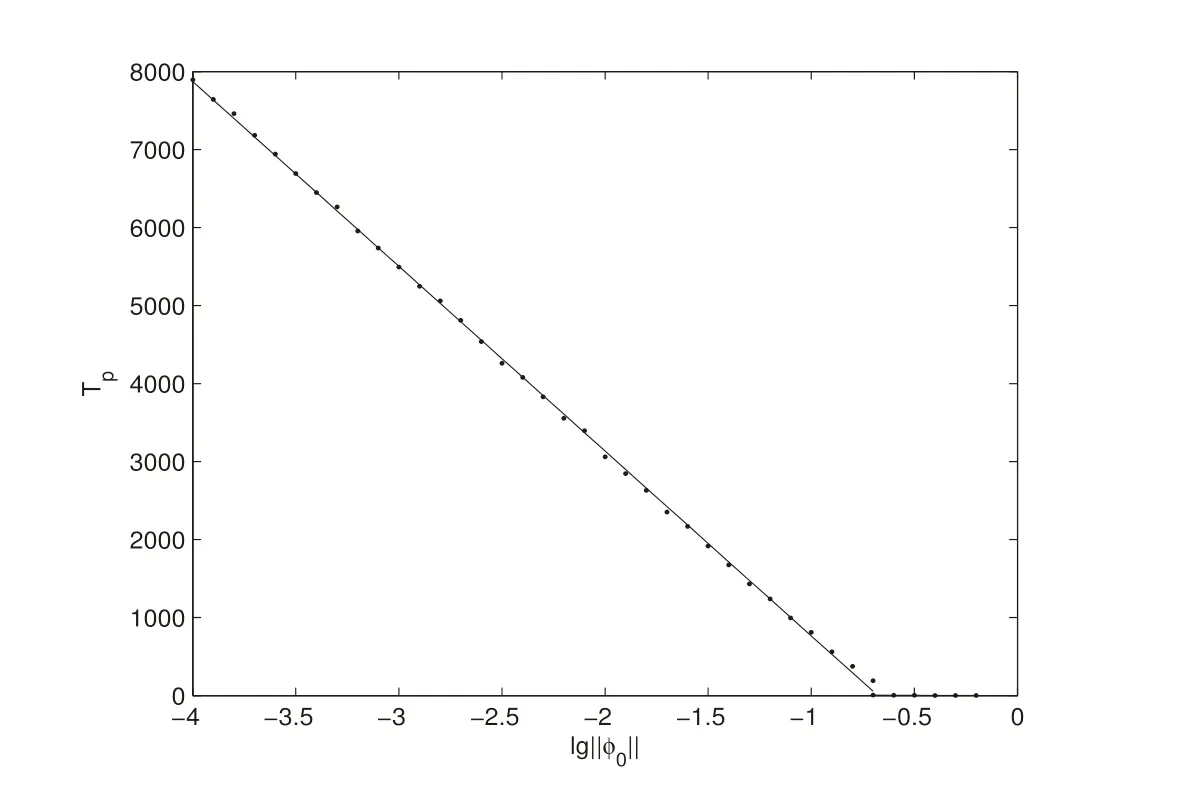
Figure 19:Dotted line:scatter diagram of Tp and lg‖φ0‖;Full line:numerical simulation result of the relationship between Tp and lg‖φ0‖

The logarithmic relationship implies that Tpis unbounded as φ0approaches 0.The time of validity of the TLM can be extended as long as we can reduce the initial perturbation.

6 Conclusions

In this paper,a new objective function‖Mn(Φ0+φ0)-Mn(Φ0)-Ml(φ0)‖is defined to combine the nonlinear mechanism of amplification of initial perturbations and the TLM of the nonlinear model for studying the validity of the TLM,so that the validity can be described more precisely.We obtained some estimates of parameters numerically about the validity of the TLM for the Lorenz equations.Finally we obtain the confidence interval to expand the scope of the relevant parameters.In fact,the validity of the TLM is affected strongly by the initial states in the Lorenz model.Our result suggests that the limit of the time prediction of validity of the TLM can be extended as long as the initial error can be reduced.

Acknowledgement:This project is Supported by the National Natural Science Foundation of China(Grant Nos.11471166 and 11426134),the Natural Science Foundation of Jiangsu Province(Grant No.BK20141443).