Mustafa Turkyilmazoglu

Abstract: A ratio approach based on the simple ratio test associated with the terms of homotopy series was proposed by the author in the previous publications. It was shown in the latter through various comparative physical models that the ratio approach of identifying the range of the convergence control parameter and also an optimal value for it in the homotopy analysis method is a promising alternative to the classically used h-level curves or to the minimizing the residual (squared) error. A mathematical analysis is targeted here to prove the equivalence of both the ratio approach and the traditional residual approach, especially regarding the root-finding problems via the homotopy analysis method. Examples are provided to further justify this. Moreover, it is conjectured that every nonlinear differential equation can be considered as a root-finding problem by plugging a parameter in it from a physical viewpoint. Two examples from the boundary and initial and value problems are provided to verify this assertion. Hence, besides the advantages as deciphered in the previous publications, the feasibility of the ratio approach over the traditional residual approach is made clearer in this paper.

Keywords: Homotopy analysis method, convergence control parameter, optimum value, ratio approach, residual approach.

1 Introduction

Homotopy analysis method (HAM) has been an attractive powerful method in the recent literature for obtaining the analytic approximate solutions of really challenging and highly nonlinear equations arising from the real-life physical applications. Many such mathematical models were treated by the method, one can refer to the books [Liao (2003),2012, 2014)], published by Liao; the founder of the method. Particularly, the "steadystate" resonant waves not detected by traditional analytic methods in the past 60 years were successfully discovered by HAM in Liu et al. [Liu and Liao (2014)], whose physical existence was also approved via a recent experiment in Liu et al. [Liu, Xu, Li et al. (2015)].The so-called convergence control parameter constitutes the cornerstone of the HAM,since it ensures the convergence of the method,whose absence may lead to an inevitable divergence in,for instance the special case of HAM;the homotopy perturbation method.Therefore,determination of a suitable value for the convergence control parameter,even finding an optimal value for it to get the fastest convergence rate are open problems in the HAM.The researchers working in the field,either make use of the out of date notion of h-level curve analysis,from which an appropriate value of convergence control parameter is tried to be picked up by observing the trend of the curve.Or,as introduced in Liao[Liao(2010)],the conventional minimization of the error through the squared residual may yield an optimum value for the convergence control parameter within a spotted interval.Such an approach is also beneficial for sorting out the applicable range of physical parameters in nonlinear physical models,refer to Turkyilmazoglu[Turkyilmazoglu(2016)].

A completely new proposal was made by Turkyilmazoglu(see Chapter 5 in the book by Liao[Liao(2014)]),based on the simple ratio test of the homotopy series terms produced as a result of HAM method.Accordingly,the proposal was shown to not only generate the same optimum convergence control parameter like the one from the squared residual approach,but produce the same interval for the convergence control parameter like the one from the h-level curve analysis.Besides,more importantly,the novel ratio approach was used to pursue the convergence of the method itself.All these and further advantages were clarified in the recent publications by Turkyilmazoglu[Turkyilmazoglu(2015,2018)].

Homotopy analysis method has been frequently used lately in the literature to solve highly nonlinear mathematical models. For example,the nanofluid problem in a channel with MHD effects was investigated by Sheikholeslami et al.[Sheikholeslami and Ganji(2014)].Hetmaniok et al.[Hetmaniok,Slota,Witula et al.(2015)]used it to solve the one-phase inverse Stefan problem.It was also used to explore the multi-valued behavior for a twolevel system by Aquino et al.[Aquino and Boot(2016)].Curato et al.[Curato,Gatheral and Lillo(2016)]suggested a discrete homotopy analysis for solving the nonlinear transient market problem. Nonlinear oscillations of micro/nano beams were simulated with the method given by Roozbahani et al. [Roozbahani,Arani,Zand et al.(2016)].Slip flow effects were examined via the method by Sravanthi[Sravanthi(2018)].The backward heat conduction problem was treated by the homotopy analysis method by Liu and Wang[Liu and Wang(2018)].Homotopy analysis method was also successfully used for treating the nonlinear equations arising from the channel flow,see Rana et al.[Rana,Shukla,Gupta et al.(2019)]. Fractional differential equations are also easily treated by the homotopy analysis method,see Martinez et al. [Martinez and Aguilar(2019)]. Very recently,the convergence of homotopy solution via Banach fixed point theorem approach was presented by Abbas et al.[Abbas,Kitanov and Longo(2019)]concerning the Lane-Emden problem.The motivation in the present investigation is to supply a mathematical analysis to prove the equivalence of both the residual and the ratio approaches concerning the convergence control parameter on the problems of root-finding by means of HAM.It is also asserted that boundary and initial value problems may be considered as a root-finding problem by inserting some parameters in them from a physical standpoint. Moreover,illuminating further advantages of the ratio approach is the main objective. Particularly when the physical domain extends up to infinity,the ratio approach seems to be more feasible as compared to the classical approaches.This is exemplified on a third-order highly nonlinear boundary value problem representing the fluid flow induced by deforming surfaces as investigatd by Liao[Liao(2005)].In addition to this,if the problem is an initial value type without an explicit interval of interest,there is no need to set up an imaginary interval on which the convergence control parameter is sought,but the ratio approach is again feasibly determining the interval of convergence control parameter and optimum value of it without a domain of definition of the physical problem. This is also demonstrated on the welldocumented van der Pol oscillator problem of physics by Chen et al.[Chen and Liu(2009)]and Abbasbandy et al.[Abbasbandy,Lopez and Ruiz(2011)].

2 The HAM and the ratio approach

The aforementioned citations are good resources for the definition of the HAM method.In summary,a convergent homotopy series solution

is sought regarding the unknown function u(t)generally satisfying a highly nonlinear differential(algebraic for the root-finding problem)equation due to the mathematical modeling of a real physical phenomenon.The parameter h appearing in(1)represents the so-called convergence control parameter determination of whose value is of the paramount significance in the present research.

In practice,the truncation of the homotopy series(1)at the order M will suffice to get an Mth-order approximate analytic solution

As a consequence of the Theorem given by Liao[Liao(2014)](see Chapter 5 in Liao[Liao(2014))],it was conjectured that under a proper choice of norm(L2norm unless otherwise is stated),the ratio defined by

will provide the necessary information for both the convergence and optimal value for the convergence control parameter h of the homotopy series(1),in such a manner that(3)is forced to be minimized(as small as possible,always being less than unity)in the large M limit.

It was shown by Liao[Liao(2014)]and Turkyilmazoglu[Turkyilmazoglu(2015)]that the interval of convergence control parameter h obtained by the constant h-level curves is considerably recovered by the ratio(3),nonetheless this is an only a local event,from which the optimum value cannot be located.Nevertheless,if we are interested in the root-finding problem like f(u)=0,the version of(3)

and β ＜ 1 for sufficiently large M will enable us to determine the interval of the convergence control parameter as well as its optimal value by minimizing(4).

On the other hand,the traditional approach is to minimize the squared residual error

and reach an optimal value of h as a result,for a given nonlinear problem N[u(t)]=0.

Hence,on a suitable domain of definition,either(3)or(5)(or their discrete versions as defined by Liao[Liao(2014)]and Turkyilmazoglu[Turkyilmazoglu(2015))]can be made use of finding the optimal convergence control parameter h. The advantages of ratio approach(3)over the squared residual approach(5)were discussed by Liao[Liao(2014)]and Turkyilmazoglu[Turkyilmazoglu(2015)]on a variety of physical phenomena.However,the question of gaining the same optimal value of convergence control parameter from both(3)and(5)is yet to be answered which is the prime objective here.Moreover,there exist two further questions in the squared residual approach;regarding the boundary value problems having an infinite interval,how the integrations will be performed either analytically or numerically in(5)is not clear.This is generally accomplished by setting the infinity at a finite cut.Also,regarding the initial value problem how a proper definition of the domain will be chosen is not known.Generally,an arbitrary finite region is set by the user.These issues are discussed and exemplified in the coming sections.

3 Root-finding problems

Theorem.Let the homotopy series

be the solution of the root-finding problem

Then,the optimum value of convergence control parameter h as obtained from the residual

coincides with the optimum value of convergence control parameter h as obtained from the ratio

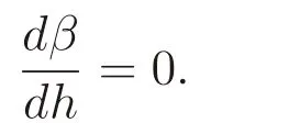
Proof.Minimizing(7)leads to an optimum h satisfying

Differentiating(6)term by term together with the consideration of(9)results in

This clearly implies that series in(10)which is the derivative of the homotopy series(6)with respect to h is convergent,therefore,

This obviously means that the optimum h of the residual(7)is also the optimum h of the ratio(8),because at such a h it holds that

This completes the proof.◇

3.1 An algebraic equation

Suppose it is desired to find the roots of

Figure 1:h-level curves for Eq.(12)

Table 1:Root of(12)and absolute errors for various M at h=-0.36. a Solutions from the homotopy method(2)and b Solutions from the Newton iteration method(15)

one of which has an exact value=0.6180339887.With the choices of initial and auxiliary variables and referring to the homotopy given in the references Liao [Liao (2014)] and Turkyilmazoglu[Turkyilmazoglu(2015)],we define the residual and absolute errors at the Mth-order homotopy approximation(2)in the forms

The convergence control parameter h versus the root of(12)and its interval of nearly h ∈[-0.5,0)are depicted in Fig. 1 at some selected approximation levels M. The range of convergence parameter(and its bounds)is seen to settle down as M increases.Actually,the exact intervals of convergence,though cannot be identified in Fig.1,solving the inequality(4)gives rise to exact intervals[-0.4647,0],[-0.4337,0],[-0.4217,0]and[-0.4146,0],respectively,at M =8,12,16 and 22,which are consistent with figure 1.Minimizing the residual in Eq. (13)and also minimizing the ratio in Eq. (4)yield the minimum value for the residual and ratio resulting in approximately h=-0.36 at the 22th-order homotopy approximation,as also observed from Figs.2(a)-2(b).

Figure 2: (a)Residual error(13)and(b)ratio(4)associated with Eq. (12)at the approximation level M=22

Table 2:The values of optimal h from the residual error(13)and the ratio(4).CPU times in seconds are in parenthesis.a Eq.(13)and b Eq.(4)

Taking into consideration the modified Newton iteration[Liao(2012)].

Tab.1 demonstrates the approximate root and also the absolute error from(14)by fixing the convergence control parameter at h=-0.36.It is anticipated that both methods limit towards to the same root,more significantly,the HAM solutions are more accurate than those of the classical modified Newton iteration at h=-0.36,for the tabulated iteration levels. Tab. 2 reveals the values of optimum h calculated from both the residual error(13)and the ratio(4)at several approximation orders. In line with the stated Theorem,the optimums from both approaches are tending to the same value,with a clear advantage of the ratio approach in terms of the CPU times.To further assess the convergence of the homotopy series(2)for the considered problem(12),ratios from(4)are depicted in Figs.3(a)-3(b)at two selected values of h.The figures clearly indicate the convergence of the employed homotopy technique.

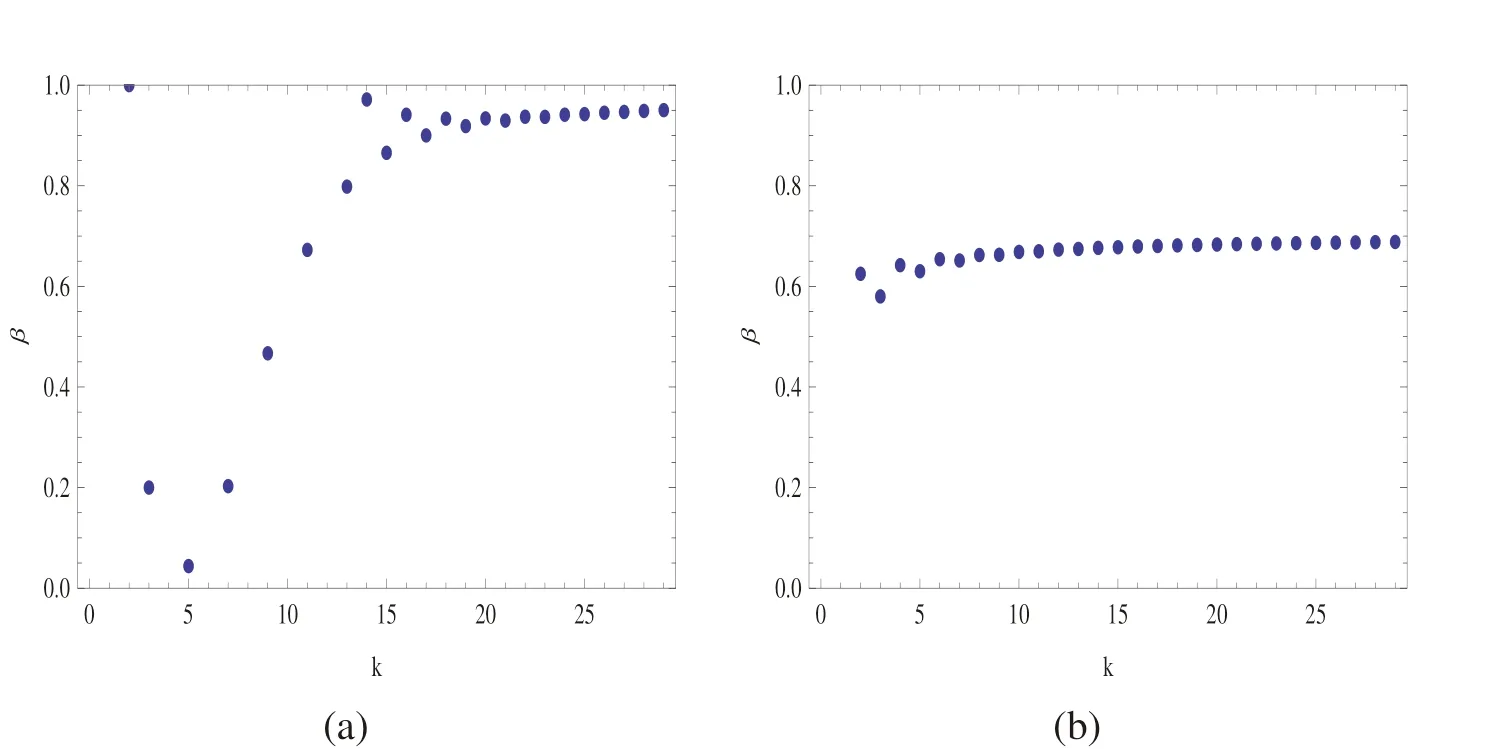
Figure 3:Ratios from(4)versus the order of homotopy approximation concerning Eq.(12)for two values of h

Table 3:The values of optimal h from the residual error(13)and the ratio(4).CPU times in seconds are in parenthesis.a Eq.(13)and b Eq.(4)

3.2 A transcendental equation

Suppose it is desired to find the root of

whose exact solution cannot be written in an elementary way.

As in the previous example,searching for an optimum convergence control parameter h from both approaches results in the values as tabulated in Tab.3.A drastic increase in the CPU time for the evaluation of residual is noticeable necessitating the use of ratio approach.It can thus be concluded that both the classical residual and present ratio approaches generate the same interval of convergence control parameters as well as the optimum values of them.Apparently,the present ratio method is desirable owing to the less time-consuming feature. Moreover,for the considered problems,at the optimum value of convergence control parameter,the present procedure is certainly more accurate as compared to the modified Newton iteration technique.However,it is still an open question whether this is the case for general root-finding problems.

4 Boundary and initial value problems

We will show in this section that the ratio approach for determining the optimum convergence control parameter in boundary and initial value problems is more feasible since it does not require a domain of interest,which must be supplied in the squared residual approach.It should be remarked that as emphasized by Liao[Liao(2014)]and Turkyilmazoglu[Turkyilmazoglu(2015)],the convergence of HAM and the optimum value of convergence control parameter are more easily accessible in the HAM method if an unknown parameter is involved in the solution.Even if no such a parameter exists,considering the unknown data from the boundaries one can always be plugged into the system.In fact,this somewhat reduces the differential equation into a root-finding problem as highlighted in the subsequent remark.

Remark.Insertion of an unknown parameter into a nonlinear differential equation converts it to a root-finding problem.Hence,the Theorem given in Section 3 enables us to work out the optimum convergence control value of h from the root in place of the classical squared residual error.

4.1 Fluid flow induced by deformable bodies

Consider the fluid flow induced by a deforming surface,having engineering and industrial applications as explored by Jaluria et al.[Jaluria and Torrance(2003)]and governed by the following third-order nonlinear differential equation[Liao(2005)].

We closely follow the homotopy study of Liao[Liao(2005)]and implement the change of variables

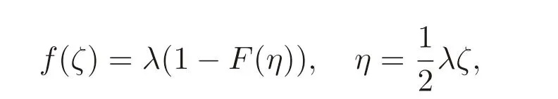
with λ=f(ζ →∞)＞0 and β ＞-1 for the physical purposes,after which system(16)turns out to be

with Γ=λ-2is unknown.

Therefore,it is aimed to obtain the homotopy series approximations for(18)

by adopting the auxiliary linear operator and the other auxiliary variables as in Liao[Liao(2005)].It is noted that the unknown values Γnwill be found to comply with the assumption of simple exponential base functions as the solutions.Moreover,out of the two solutions of Γ0as detected by Liao[Liao(2005)],we only pursue the larger one since it is inclined to be more physical.

Figure 4:h-level curves for Eq.(18)

Since F′′(0)is unknown from(18),the local range of convergence control parameter may be determined from the plot in Fig.4(a),suggesting that as the order of approximation is increased,the interval of convergence is approximately thought of[-1,0].Making use of the ratio in(3)for F′′(0)and accounting for the inequality

We find that (19) yields the exact intervals

[-0.8124, 0], [-0.9205, 0], [-0.9122, 0], [-0.9051, 0]

at the approximation orders M = 9, 15, 23 and 31, respectively, which are very close to the intervals estimated by the h-level curves in Fig. 4(a). The almost same intervals of convergence control parameter h can also be observed in Fig. 4(b) from the ratio

and imposing β ＜ 1 in (20) yields the exact intervals

[-0.9482, 0], [-0.9292, 0], [-0.9154, 0], [-0.9009, 0]

at the approximation levels M = 9, 15, 23 and 31, respectively. The advantage here is that producing Fig. 4(b) takes much shorter time (within 20 seconds) than producing Fig. 4(a)(over 10 minutes) since functional series are involved in the evaluation of F′′(0).

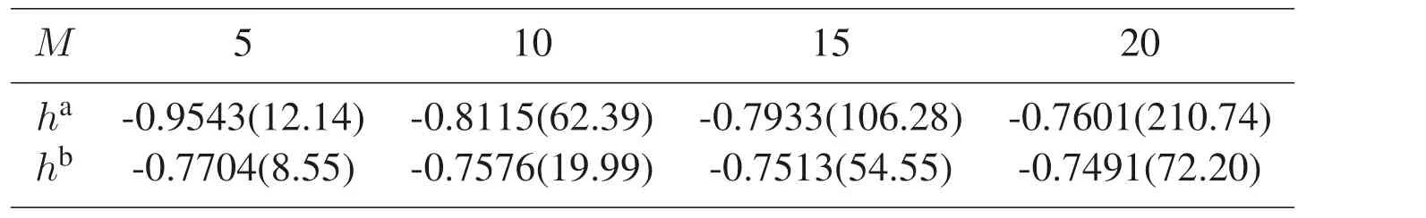
Table 4:The discrete values of optimal h from both approaches for Eq.(18).CPU times in seconds are in parenthesis.a From Eq.(5)and b From Eq.(3)

As mentioned in Section 2,one of the main drawbacks of the squared residual error is in the calculation of integrals in(5)whether analytically(almost impossible for the current problem)or numerically.The infinite domain is another difficulty for the squared residual,even though ratio can be analytically computed from(3)up to some level of approximations.By setting infinity at η=10 and choosing 50 equi-spaced points in the reduced domain[0,10],discrete squared residual for(5)and discrete ratio for(3)result in the better range of convergence control parameter h and also an optimum for that of approximately h=-0.75 as also demonstrated in Figs.5(a)-5(b).

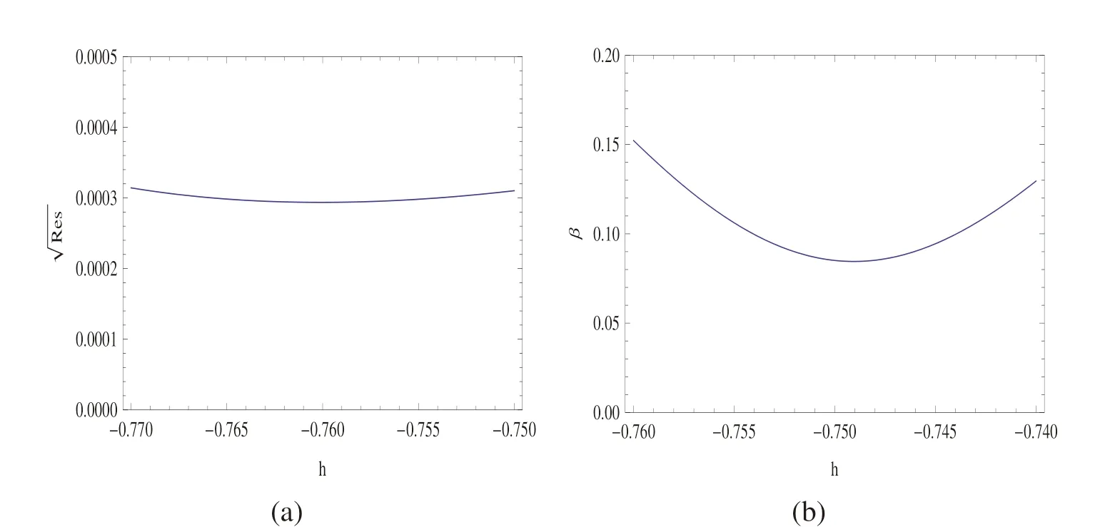
Figure 5:(a)Residual error(5)and(b)ratio(3)for Eq.(18)at approximation level M=20

Tab.4 also tabulates the information regarding the optimum h values from both squared residual and ratio approaches and the CPU times in seconds.

Instead,minimizing the ratio associated with Γ in Eq.(20)as listed in Tab.5 does not take even a minute,refer also to Fig.6.Hence the ratio approach is indeed superior for the current problem in identifying a proper convergence control parameter.

To further check out the convergence of the homotopy series solution for the current problem,the ratios are plotted at three different values of h in Figs. 7(a)-7(c)from(3)and in Figs.8(a)-8(c)from(20).Since the ratios approach a finite limit in each case less than unity,the convergence of the homotopy solution is assured. We may conclude in thissection that the semi-infinite problems hardening the location of an optimum convergence control parameter via the classical squared residual error is overcome by the introduction of a free parameter into such systems and tracing that parameter within the presented ratio approach.

Table 5:The exact values of optimal h from the ratio(20)for Eq.(18)

Figure 6:Ratio(20)for Eq.(18)at several approximation levels

4.2 Van der Pol oscillator

The traditional van der Pol oscillator problem is given by the subsequent nonlinear secondorder differential equation,as investigated by Chen et al. [Chen and Liu(2009)]and Abbasbandy et al.[Abbasbandy,Lopez and Ruiz(2011)]

modeling the phenomena of many problems of vibration whose amplitude is A,refer to the publications Dafear et al.[Dafear,Geer and Andersen(1984)]and Buonomo[Buonomo(1998)]. By means of the transformation τ =Ω t,where Ω is the frequency of the oscillations,Eq.(21)is now

Figure 7:Ratios from(3)for Eq.(18)with various h

In(22)both Ω and A will be treated as unknowns,which will be determined as a result of removal of secular terms,by assuming a homotopy series solution of(22)in the form

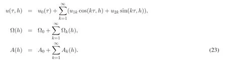
Such a solution is achieved following[Chen and Liu(2009)]and[Abbasbandy,Lopez and Ruiz(2011)]by the auxiliary variables

Figure 8:Ratios from(20)for Eq.(18)with various h

The h-level curves are displayed in Figs. 9(a)-9(b) to determine the interval of convergence of h, from the unknown u′′(0), Ω and A, respectively. The convergence of the HAM solutions in(23)appears to take place at the interval[-1.5,0]according to these figures. This is also analytically derived;an exact interval of[-1.1415,-0.0425]is obtained using(3)for u′′(0),the interval of[-1.2740,0]using(4)for Ω and the interval of[-1.2621,-0.0403]using(4)for A at the homotopy approximation level M=24.

At this level it is found that the optimum value of h is approximately h=-0.93 from the squared residual(5)(taking the integration domain[0,2π]and numerical integration by 50 equi-spaced points),from the ratio(19)for u′′(0)and from the ratio(20)associated with Ω and A as seen from Tab.6.Tab.7 further tabulates the frequency and amplitude corresponding to h=-0.93 at various approximation levels.Considering that the exact values are Ω=0.9429558474 and A=2.0086198609 from the publication Chen et al.[Chen and Liu(2009)],the accuracy of the gained HAM solutions is acceptable.In order to further justify the obtained homotopy series solutions for the current problem,Figs.10(a)-10(b)show the vibration behavior of van der Pol oscillator(21).It is noted that the exact solution is given at A=2.0086198609 shown by thin curves,whereas dotted curves correspond to initial approximation,dot-dashed curves to first-order HAM solutions and dashed curves to 5th-order HAM solutions.

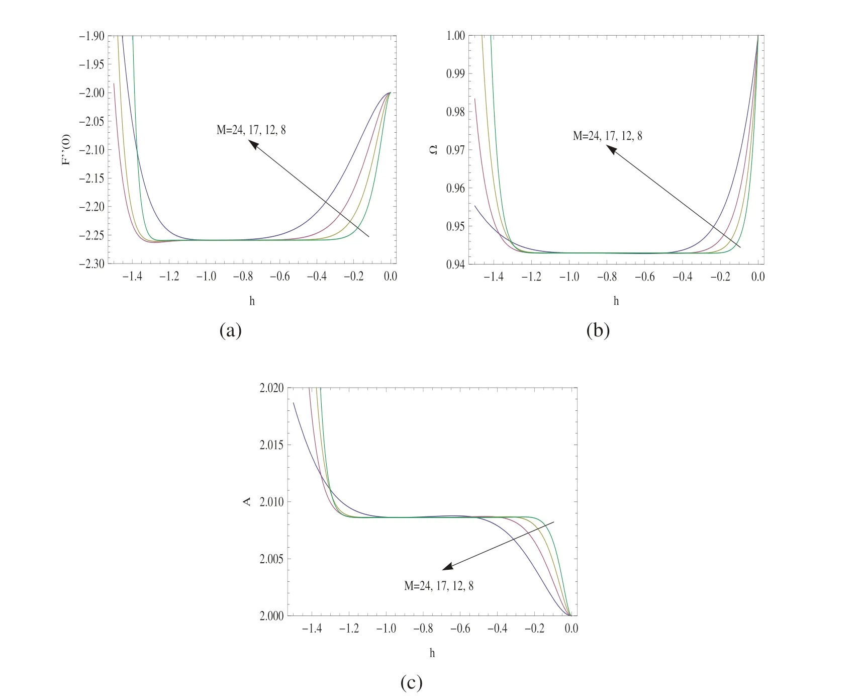
Figure 9:h-level curves for Eq.(22)

Table 6:The optimum values of h evaluated by minimizing discrete squared residual(5),the ratio(19)for u′′(0)and the ratio(20)for Ω and A. CPU times in seconds are in parenthesis.a Eq.(5)and b Eq.(19)for u′′(0),and c Eq.(20)for Ω,and d Eq.(20)for A

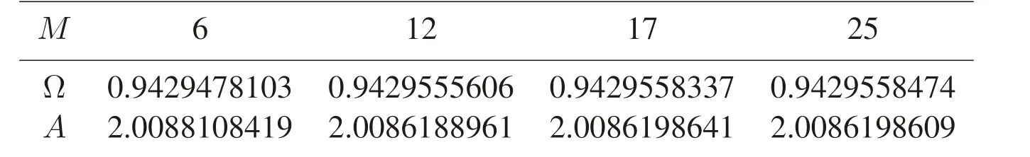
Table 7:The frequency Ω and amplitude A with h=-0.93

Figure 10:Views from the van ver Pol oscillator(21).The full solution is shown by thin curves,the initial approximation is by dotted curves,the first-order HAM solutions by dotdashed curves and the 5th-order HAM solutions by dashed curves

Hence,we may conclude that in parallel to our assertion,there is no need to set up any physical interval as in the current initial value problem,but simply use the ratio approach to accurately predict the convergence control parameter h from which physical insight can be gained for the considered problem. We should finally remark that the ratio approach can also be beneficial to apply to more complicated partial differential equations, especially if they contain a free parameter. Otherwise, the traditional residual error minimizing would require much extensive CPU time due to the evaluation of multiple integrals over the physical domain of considered problem in bounded or unbounded types.

5 Concluding remarks

The present work is devoted to the determination of convergence control parameter frequently needed in the homotopy analysis method. The recently proposed simple method of ratio, in the publications, Liao [Liao (2014)] and Turkyilmazoglu[Turkyilmazoglu (2015)], based on the classical calculus is the main focus here. It was shown in the latter that the ratio approach has certain definite advantages for identifying the optimum convergence control parameter in the homotopy analysis method, and it constitutes a promising alternative to the classical h-level curve analysis or to the minimizing the squared residual error. A rigorous proof is given here to show that both the ratio approach and the traditional residual approach result in the same optimum value for the convergence control parameter in solving the algebraic equations. Two examples are provided to support this fascinating outcome. It is later conjectured that any boundary or initial value problem may be considered as a root-finding problem by inserting unknown parameters from the physical boundaries. The feasibility of the ratio approach is then exhibited on some selected fashionable initial and boundary value problems by inserting unknown parameters into the system and tracing the ratios from these parameters, in place of the more time-consuming definition of the ratio. Such an approach seems necessary for the physical problems possessing infinity domains since the classical squared residual approach may not be trustable even when the discrete version of it is employed. In addition to this, if the problem is an initial value type, without an explicit interval of interest, there is no need to set up an imaginary interval on which the convergence control parameter is sought, but the ratio approach is again feasible determining the interval of convergence control parameter without a domain of definition of the physical problem.The presented physical examples from the deformable surfaces and the van der Pol oscillator justify the assertions made here. To conclude, the advantageous ratio approach may be safely used to determine the interval and optimum convergence control parameters in the future applications of the HAM method taking into account more complicated mechanical and engineering problems in nonlinear science [Hashemi (2015)].

Acknowledgement:The author wish to express his appreciation to the reviewers for their helpful suggestions which greatly improved the presentation of this paper.