,

(School of Mathematical Sciences, University of Chinese Academy of Sciences, Beijing 100049, China)(Received 26 September 2017： Revised 4 January 2018)

Abstract In this work, we propose a Lie algebraic approach for numerically solving a class of highly oscillatory stochastic Hamiltonian systems (SHSs). For a concrete highly oscillatory SHS, we construct two numerical schemes based on the Lie algebraic approach, and prove their near preservation of the symplecticity. We also show by numerical tests their root mean-square convergence orders, as well as their effectiveness and merits in solving the highly oscillatory SHS.

Keywords numerical solutions of stochastic differential equations; stochastic Hamiltonian systems; highly oscillatory SDEs; operator splitting methods; Lie algebraic approach

Stochastic differential equations (SDEs) play an important role in the description of phenomena in many subjects[1-2], such as biology, mechanics, chemistry, and microelectronics. The Hamiltonian system is one of the most important dynamical systems. All the real physical processes where the dissipation can be neglected can be formulated as Hamiltonian systems[3]. Stochastic Hamiltonian systems (SHSs) are the Hamiltonian systems with stochastic disturbances.

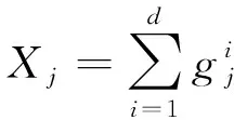
A 2n-dimensional SHS can be written as the SDE of Stratonovich sense[4-5]with initial valuesP(0)=p,Q(0)=q,

(1)

wheref,g,σr, andγr,r=1,…,m, aren-dimensional column vectors, andWr(t),r=1,…,m, are independent standard Wiener processes. There are functionsH(t,P,Q),Hr(t,P,Q)，r=1,…,m, such that

fi=-∂H/∂qi,gi=∂H/∂pi,

(2)

Similar to deterministic Hamiltonian systems, the phase flow of SHS (1) preserves the symplectic structure characterized by

,∀t≥0, a.s.,

The exact solutions to SDEs are in general very difficult to obtain. Therefore numerical methods become important tools for simulating solutions to SDEs. In recent decades, there arose many studies regarding different aspects of numerical methods of SDEs[6-8]. The study of numerical solutions for highly oscillatory problems is an important branch, to which many works were devoted, such as Refs.[9-12]. Standard numerical methods are usually not suitable for treating such problems tecause they require very small time step sizes and thus make the computations prohibitively expensive.

In this work we focus on the stochastic highly oscillatory problem with initial valuesP(0)=p,Q(0)=q,

dP=(-1-f(P,Q))Qdt-σQ∘dW(t),

dQ=(--1+f(P,Q))Pdt+σP∘dW(t),

(3)

(4)

Our motivation is to employ the Lie algebraic approach to solve this class of highly oscillatory SHSs (3) with conditions (4), and we establish two numerical schemes for a concrete highly oscillatory SHS based on the Lie algebraic approach. Further, we analyze the symplecticity of the two schemes and prove that they nearly preserve the symplectic structure. Next we investigate their root mean-square convergence orders, efficiency, and superiority via numerical experiments.

1 The Lie algebraic approach

Let (Ω,F,{Ft}t≥0,P) be a complete probability space with filtration {Ft}t≥0. Consider the SDE of Stratonovich sense under the probability space (Ω,F,{Ft}t≥0,P), with initial valueS(0)=s0,

∘dWj(t),

(5)

whereb,gj,j=1,…,r, ared-dimensional∞functions andW(t)=(W1(t),…,Wr(t)) is am-dimensional standard Wiener process. Define the∞vector fields

(6)

where ∂i=∂/∂Si. There is a representation theorem in Ref.[14] for the solution of SDE (5), which is the base of the Lie algebraic approach. To state the theorem, we first introduce some notations.

Given a multi-indexJ=(j1,…,jm) and [X,Y]=XY-YX,XJis defined as

XJ=[[…[Xj1,Xj2],…],Xjm].

=(J1,…Jk1)(Jk1+1,…Jk2)…(Jkl-1+1,…Jkl).

(7)

(8)

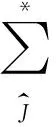
whereW0(t)=t. For a double divided index,

(9)

where

Lemma1.1Suppose that the Lie algebraL=L(X0,X1,…,Xr) generated byX0,X1,…,Xris nilpotent of stepp. Then the solutionS(t) of (5) withS(0)=sis represented asS(t)=exp(Yt)(s), whereYt(ω) is the vector field given by

(10)

almost surely for eacht.

×

(11)

Given a time discretization {tn} of the interval [0,T] with an equidistant step sizeh, i.e.,tn=nh,n=0,1,…,N. The Lie algebraic approach to construction of numerical methods follows the procedure[2]as follows.

•Based on the representation of the solution of the SDE (5), write the time discretization schemeSn+1=exp(Yn,h)(Sn);

•After obtaining a truncated vector fieldn,hby discarding the higher order terms, construct the truncated schemen+1=exp(n,h)(n);

2 The Lie algebraic methods for highly oscillatory SHSs

Now let us consider the highly oscillatory SDE (3). Letf(P,Q)=P2+Q2and the dimension of the systemd=2, i.e.,

dP=(-1-(P2+Q2))Qdt-σQ∘dW(t),

dQ=(--1+(P2+Q2))Pdt+σP∘dW(t).

(13)

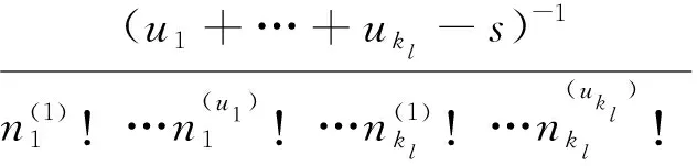
According to the conditions (4), it is clear that (13) is an SHS, with Hamiltonian functions

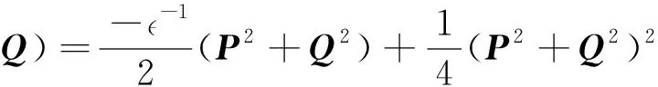
Therefore, (13) is a highly oscillatory SHS.

Performing the change of variables=t/in (13), we get the equivalent system of (13)

dP=(1-σQ∘dW(s),

dQ=(-1+σP∘dW(s).

(14)

It is not difficult to see that (14) is also an SHS. Now we apply the Lie algebraic approach to system (14), for which

X0= (1-(P2+Q2))Q∂P+

(-1+(P2+Q2))P∂Q,

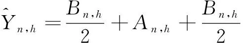
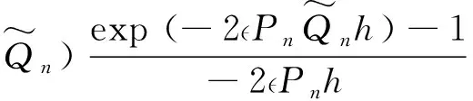
An,h=((1-σQΔWn)∂P,

Bn,h= ((-1+(P2+Q2))Ph+

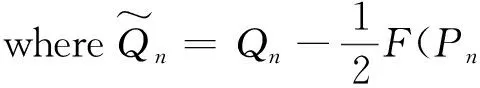
For simplicity, we denoteF(p,q)=(1-σΔWn. If we choose the operator splittingn,h=An,h+Bn,h, we get the scheme

(15)

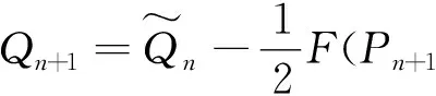
(16)

Theorem2.1The Lie algebraic schemes (15) and (16) for the highly oscillatory SHS (14) nearly preserve the symplectic structure with error of root mean-square order 3/2, i.e.,

(17)

Proof(17) holds if and only if

(18)

□

3 Numerical experiments

In this section, we illustrate the performance of the Lie algebraic schemes via numerical tests. Throughout the section, the reference solution is computed by high-order schemes with a sufficiently small step size.

In Fig.1(a) we show the sample trajectories of the numerical solutions (15) (blue), (16) (yellow), and a trigonometric integrator in Ref.[11] (green) for the highly oscillatory SHS (13), with the initial valuesp=0,q=1 and the parameters=0.01,σ=0.3, ont∈[0,1]. The step size ish=2-5. The blue and yellow lines coincide visually with the red line which is the sample trajectory of the reference solution. Hereby we construct the two schemes (15) and (16) by involving the time-rescaling change of variable in our Lie algebraic methods, on the equivalent but time-rescaled system (14) of (13), and we apply the trigonometric method directly to (13) to draw the green line, with the same time step sizeh=2-5.

In Fig.1(b) is the sample trajectory of the Lie algebraic scheme (15) under a higher frequency parameter=0.001, which is also visually in good coincidence with the reference solution. The initial values arep=0,q=1. We takeσ=0.3 and the step sizeh=2-5.

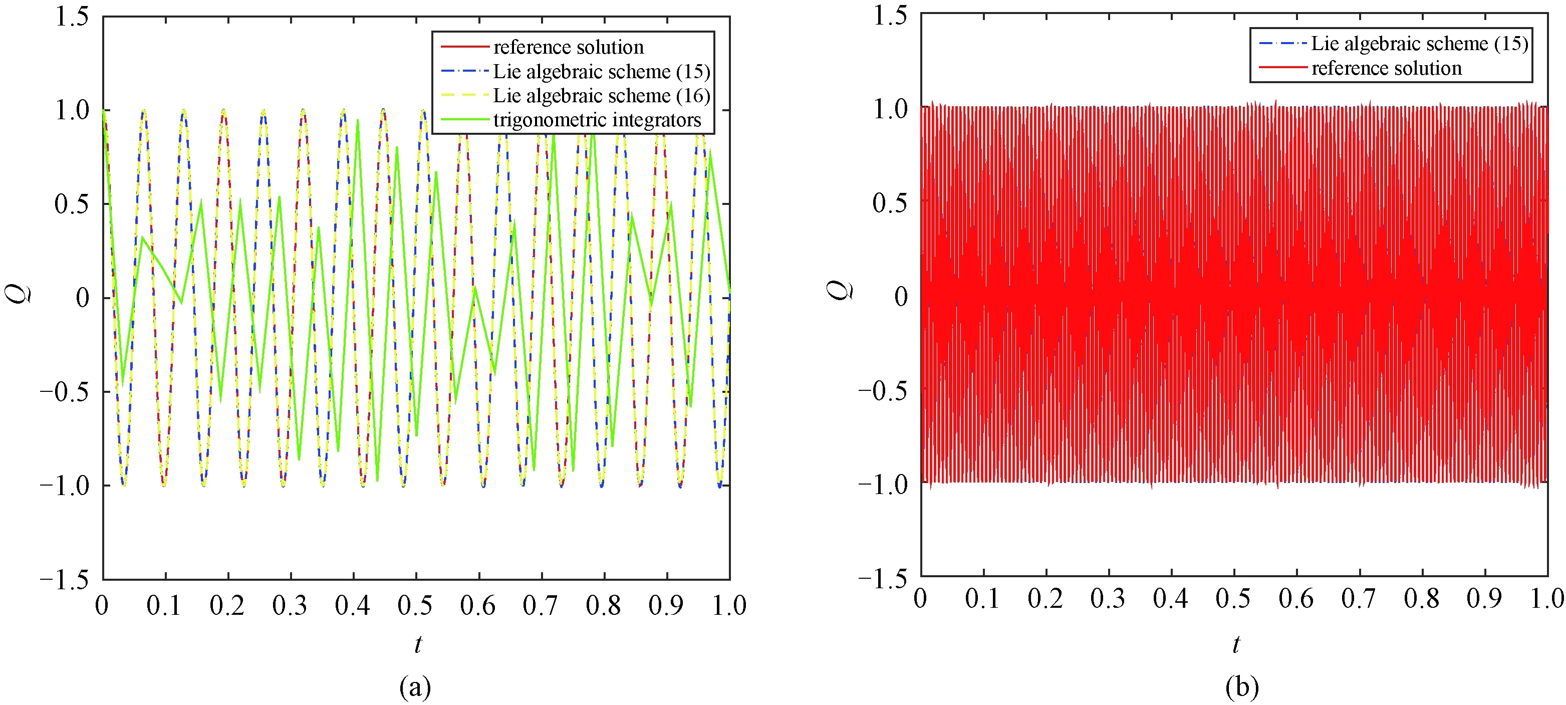
Fig.1 The sample trajectories

In Fig.2(a) and Fig.2(b) we show the preservation of the invariant quantityP(t)2+Q(t)2=p2+q2of system (13)[10]by the two Lie algebraic schemes.

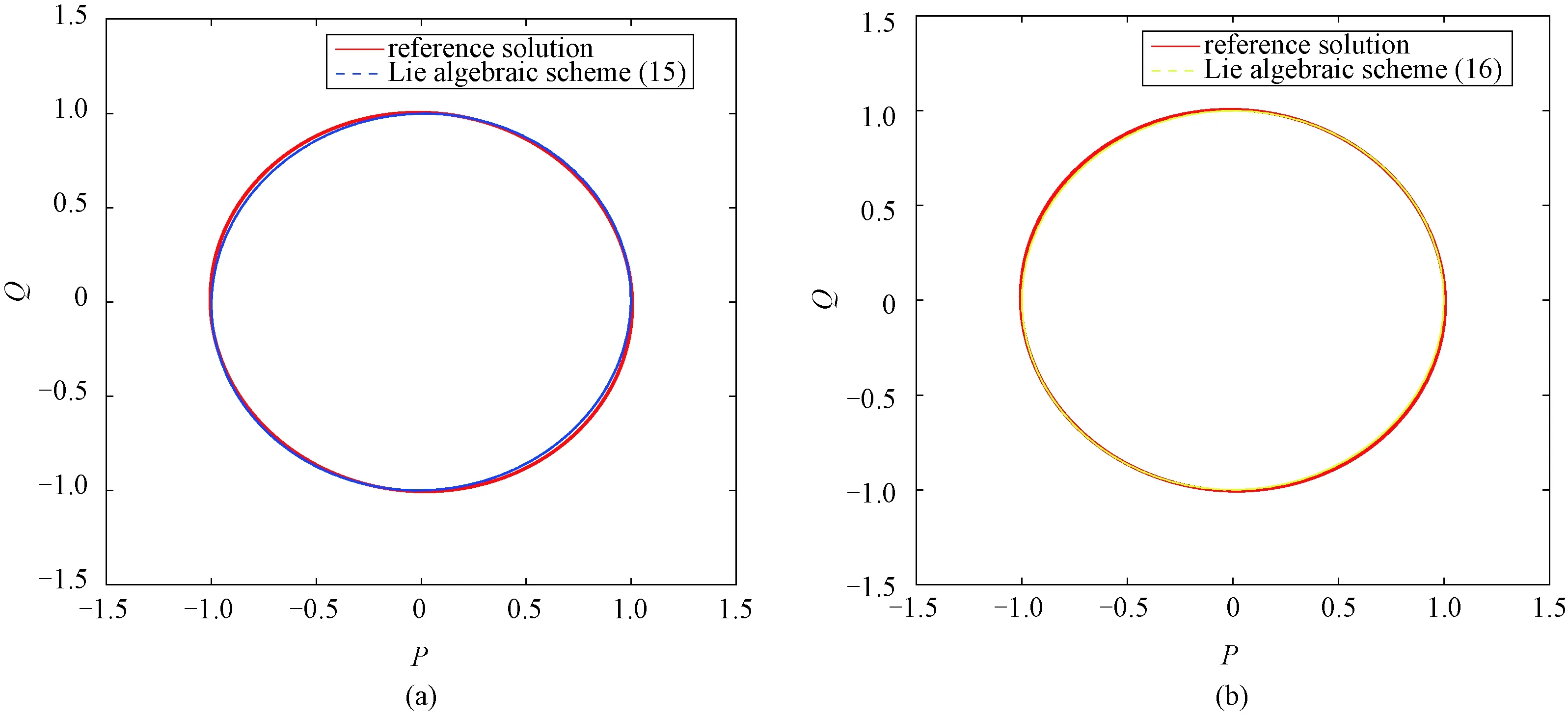
Fig.2 The phase trajectories

In Fig.2, the initial valuesp=0,q=1 and the parameters=0.01,σ=0.3. The step size ish=2-5.

As shown in Fig. 3(a) and Fig. 3(b), the root mean-square convergence orders of the Lie algebraic schemes (15) and (16) are both 1. Here we compute the error atT=1 and takep=0,q=1,=0.01,σ=0.3. Five hundred trajectories are sampled for approximating the expectation.

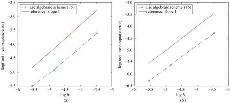
Fig.3 The convergence orders