(College of Meteorology and Oceanology,National University of Defense Technology,Changsha 410073,China)

Abstract:By the zero-frequency characteristic of the three-dimensional translating-pulsating source Green function in frequency domain,mathematical representation of a new kind of translating source is obtained with the summation of near-field flow disturbance,far-field wave component,Rankine source and its mirror of undisturbed water plane.In comparison with common representations of translating source,it is free of the infinite discontinuity and halved the integral interval,which indicates that it may achieve some numerical advantages in the wave-making resistance and steady waveprofile problems.For the near-field and far-field terms of the Green function,variable-step size adaptive Simpson algorithm and mathematical transformation method are respectively adopted to improve the stability of numerical integration.In light of the integral difficulties of the newly introduced complex function,three strategies are implemented such as the limited truncation of integral interval,the effective combination of integral approaches,the fast discrimination and evaluation of the fake singularity.A complete numerical integration approach of the translating source Green function is established,as both efficiency and accuracy aspects taken into account.Numerical results indicate that the proposed approach is reliable in the calculations of the translating source Green function and its partial derivatives with wide range of the field point and source point with uniform forward speed.

Key words:translating-pulsating source;translating source;numerical integration;Simpson integral method;fake singularity

0 Introduction

Recently,Green function method has gained extensive application in the hydrodynamic problems of ship and marine structure[1-4].The key point of the method is the accurate,fast and reliable calculation of the Green function.For the steady potential flow problem about a ship advancing at constant speed through calm water,of effectively infinite depth and lateral extent,two kinds of Green function are chosen in general[5].One kind is the Rankine source Green function with simple form,which is not satisfied with any boundary conditions.Therefore,the velocity potential in the field is determined by the suitable-strength source distribution on all the fluid boundaries.Another kind of Green function is the steady translating source,namely Kelvin source,which meets all the boundary conditions except for that on the body surface.Though the translating source is expressed in complicated form,it can exactly and automatically conform to the radiation condition of no steady making waves ahead of the advancing ship.As the numerical advantage in the steady potential flow theory,the latter source is applied in the predication of wave-making resistance for modern yachts[6]and multihull vessels[7].

In 1972,a weakly non-linear theory named Neumann-Kelvin was put forward by Brard[8].In the Neumann-Kelvin theory for the above-water hulls,the Kelvin source Green function is distributed on the body surface and at the water line,and then the source strength is resolved to acquire the filed velocity potential by the similar discrete way like Hess-Smith method[9].Many studies proved this theory’s effectiveness to the steady ship problem by Guevel et al[10]and Doctors and Beck[11].In order to simplify the mathematical representation of Kelvin source,Newman[12-13]transformed its original double-integral form to a single integral type,whose evaluation method was discussed in depth.Further,Noblesse et al[14-16]proposed the modification,called Neumann-Michell theory,of the classic Neumann-Kelvin theory of ship waves.A main difference between the two theories is that the Neumann-Michell theory did not involve the line integral around the mean water line of the ship hull surface.For the Kelvin source Green function and its partial derivatives in Refs.[17-18],the singularity and highly oscillatory of the integrand exert great influence on the precision and efficiency by direct numerical integration,and bring barrier to its application to calculate the wave-making resistance and steady ship motion.The rapid and stable integral calculation of the Green function had been carried out by Iwashita and Ohkusu[19],Newman and Clarisse[20]and Watanabe[21].However,the singularity characteristic has not yet acquired sufficient dexterity to deal with effectively if both the source and field points are close to the water surface.

If the 3-D translating-pulsating source Green function is put in the limited condition with zero frequency and nonzero advancing speed,a new mathematical representation of 3-D translating source can be achieved in a single integral form,which is the main work of present paper.The integral expression of this translating source Green function is very simple and its integrand is free of the infinite discontinuity in the whole integral interval.The behaviors of integrand are deeply explored and an accurate and stable integration method is proposed from the purely numerical perspective.This Green function is so advantageous in numerical calculation that it is expected to widely apply to the hydrodynamic problems of ship and marine structure with uniform advancing speed in calm water.

1 Fundamental mathematics

Supposing that p （ x,y,z）is a field point,andis a source point advancing at a uniform speed U and oscillating at a frequency ωe.The 3-D translating-pulsating source Green function in frequency domain can be written as follows[22-23]:

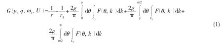
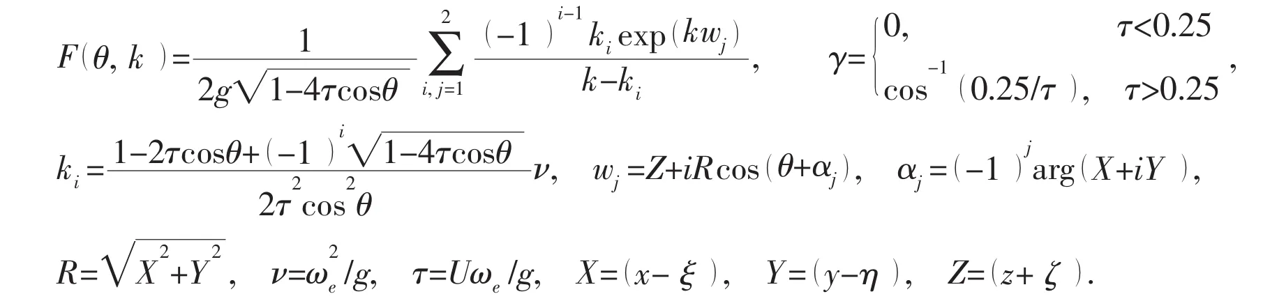
The Green function above is in a double-integral form,whose integrand and relevant parameters are defined as:

The integral path of equation(1)is illustrated in Fig.1,in which two singular points,k1and k2,presented on the contours L1and L2.Obviously,there is no singularity on the contour L3.

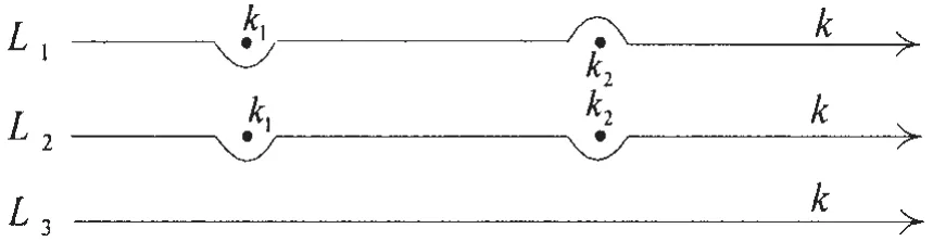
Fig.1 Integral path of the integrand about k

If the forward speed U is nonzero and the oscillating frequency ωeis zero for the 3-D translating-pulsating source Green function,it can be derived that τ=0, γ=0,k1=0,k2=g/（U2cos2θ）,the terms multiplied with k1in the integrand and the integral value on the contour L3turn to be zero.Then the representation of Green function is simplified as

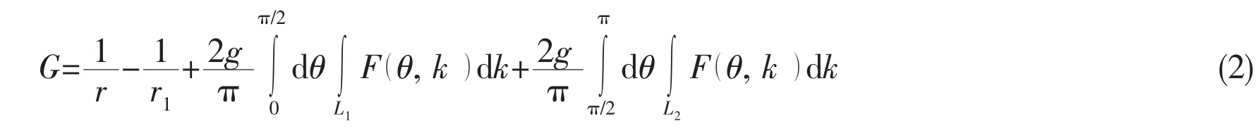
In the equation(2),the integrand can be rewritten as F=Re（F）+iIm（F）,in which Re（F）and Im（F）are the real and imaginary part of F,respectively.Eq.(3a)and(3b)presents the expressions of Re（F）and Im（F）.

where the integral values on the contours L1and L2are set as I1and I2,respectively.If the variable θ is in the interval],a transformation is introduced as θ=π-ϑ,where the new variable ϑ is fell into the intervalBased on variable ϑ,the singularity k2（θ）is corresponding toand the integral value of I2can be expressed as

According to the Eq.(3a)and(3b),the real and imaginary part of the integrand function）can be derived as

Based on the Eqs.(3a),(3b),(5a)and(5b),a notable property of F is that

In the integral path showed in Fig.1,the further transformations of I1and I2are easy to obtain as Eq.(8a)and(8b)after the introduction of Cauchy principal value integral[24].

where P.V.is the symbol of a Cauchy principal value integral and the function f（）θcan be written as follows:

By substituting the Eq.(8a)and(8b)into I1+I2,it is easy to gain that

where Re I1（）can be presented as follows according to Eq.(8a)

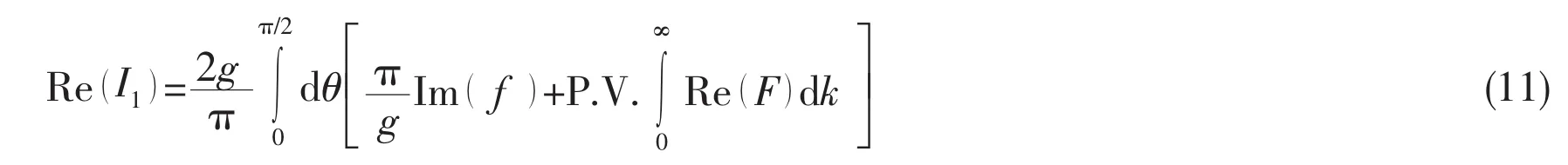
From the Eqs.(10)and(11),it is easy to obtain that I1+I2=2Re I1（）and the Eq.(2)can be further simplified as

The equation above indicates that the 3-D translating-pulsating source Green function is degraded into a real function if its oscillating frequency equals to zero,and the original three integrals about θ can be simplified as only one integral representation in the interval[0,π/2].However,the Green function in Eq.(12)is a double integral whose numerical computation is still very heavy.For the integral variable k,a linear transformation as Γ=-wj（k-k2）is then introduced[23].If a closed curve is built on the complex plane about Γ and an exponential integral function of E1（k2wj）is introduced,the representation in Eq.(12)can be rewritten as follows:

where NF is the near-field flow disturbance,and W is the wave component corresponding to the far-field wave patterns.The two terms of NF and W can be expressed as follows:

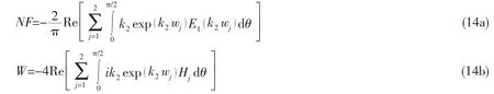
where Hjis a control factor whose value depends on the imaginary part of wjas

From the translating-pulsating source Green function in frequency domain,Eq.(13)is the mathematical representation of 3-D translating source in a single-integral form.If G*=NF+W,the partial derivatives in three directions can be presented as

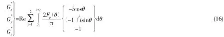
where Fp（θ）equals to

Ref.[25]expounds a kind of 3-D translating source Green function with a single integral about polar angle θ,whose disturbing term is at the summation of near-field and far-field components and integral interval isAs shown in Eq.(13),the new derivation of 3-D translating source Green function is also a single-integral,and its integral interval is halved to[0,π/2].From above all,the new representation of Green function is simple and the numerical integration is relatively light.

2 Near-field flow disturbance

2.1 Function characteristics

In Eq.(14a),there is no infinite discontinuity at the integral endpoints,which demonstrates that integral difficulty is out of infinite discontinuity for the near-field flow disturbance.The main part of the near-field flow disturbance is the production form of an exponential function and an exponential integral function.Here,the exponential integral function involves the computation of a natural logarithm,that is ln（ k2wj）.If the imaginary part of wjequals to zero,a jump discontinuity emerges for the imaginary part of ln（ k2wj）.However,the real part of ln（ k2wj）changes dramatically and shows like a peak near the jump discontinuity.Together with the horizontal distance between the field point and the source point,the peak character becomes more significant.Fig.2 shows how the integrand of near-field flow disturbance changes as the horizontal distance R with the value 10,30 and 100.More detailed parameters are that α1=π/4,α2=-3π/4,Z=0,U=5 m/s.In the condition above,the jump discontinuity θ=π/4 can be determined by the simple formula Im（ k2wj）=0.As is presented in Fig.2,a local peak starts around the point θ=π/4 and the curve with R=100 is similar to the impulse function in some degree.

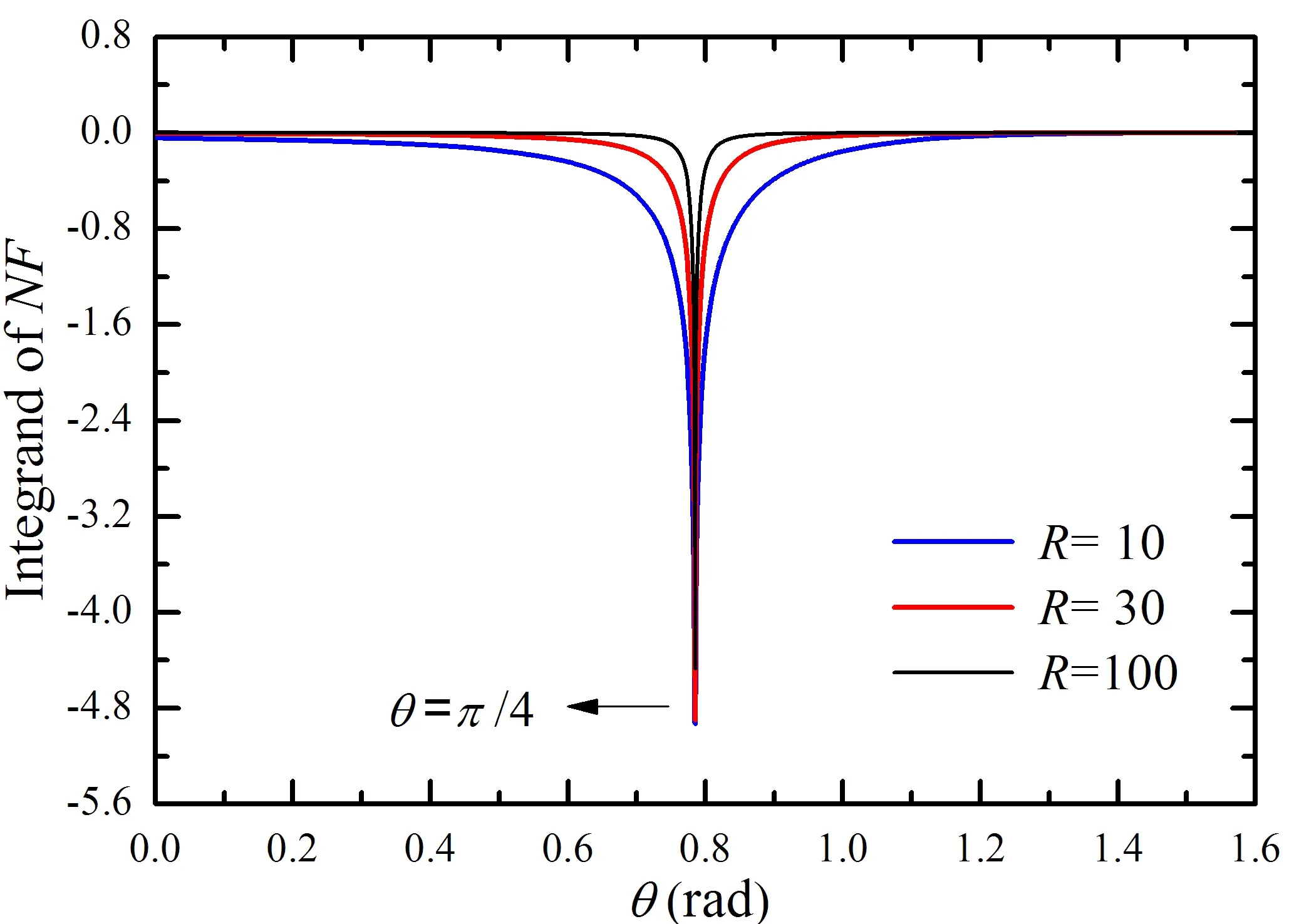
Fig.2 Integrand of the near-field flow disturbance with different value of R

2.2 Integration method

If the equal step-length integral method is implemented for the near-field flow disturbance,much more crowded discrete points need to be distributed at the jump discontinuity nearby to ensure the numerical precision.Further,the majority of the discrete points would be gathered in the interval where the integrand changes relative gently.Because of the significant waste of computational resources,the equal step-length integral method seems not the best choice for the near-field flow disturbance.Another integral method,based on the variable step-length adaptive Simpson algorithm[26],can balance the integral error for different subintervals with the whole interval.The primary advantage of the latter method is that the integration step is adjusted as the integrand’s actual trend.That is to say,a lot of discrete points can be automatically scattered where the integrand changes dramatically and less points and large step lengths adaptively distributed in the gradual interval.It can be concluded that the variable step-length adaptive Simpson integral method is well suit for the characteristics of nearfield flow disturbance.

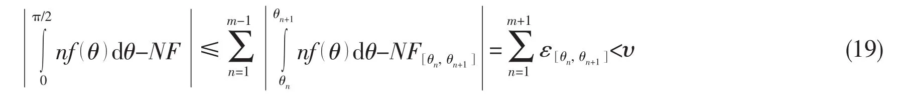
In the interval of[0,π/2],the discrete set,Δ= ｛θ1, θ2,…,θm｝,is not equidistant bearing points,in which θ1=0 and θm=π/2.In terms of variable step-length adaptive Simpson integral method,the integral error of different step-length subinterval[θn,θn+1],（1≤n≤m-1）,is approximately in line with that of the whole interval if the integral error level is defined as υ in advance.Here,the integral error is set as ε for every subinterval.As the integrand,integral interval and error level as input,an approximate integral model can be constructed in the following form:

where nf（）θis the integrand function for the near-filed flow disturbance and its expression is

In order to balance the contribution of local error from every subinterval,the following condition must be met in the interval [θn,θn+1].

So,the condition above can provide an assurance for that

3 Far-field wave component

3.1 Functional behaviors

An exponential function exp（ k2wj）is included in the integrand of the far-field wave component and its partial deviations.For k2wjis a complex number,the integrand shows oscillatory characteristics in its integral interval.By the definition of wj,exp（ k2wj）can be formulated in a more detailed form as the production of exp（ k2Z ）and exp[ ik2Rcos（ θ+αj）],where k2Z determines the oscillatory amplitude and k2Rcos（ θ+αj）represents the phase of exponential function.The wave number k2here is a monotonically increasing function about the independent variable θ.If θ goes to π/2,k2tends towards infinitude.Therefore,the integrand of far-field component oscillates with the changeable frequency in the condition R≠0 and the oscillating frequency is very high when θ tends to π/2.Another aspect is that the value of exp （ k2Z ）is decreasing gradually along with the increasing θ for Z＜0.The greater the value ofis,the smaller the oscillating amplitude of exp（ k2wj）is and more rapidly it decays.So it can be concluded that the amplitude of exponential function exp（ k2wj）oscillates to zero althoughgoes to infinitude if θ is next to π/2.

In addition,the integrand of far-field wave component is a piecewise function by the con-trol factor Hj.In part of the interval θ∈ [0,π/2],the integrand is identically equal to zero and the corresponding subinterval can be called invalid integral interval.However,the integrand does not keep at zero in some subinterval,namely valid integral interval,in which the numerical integral operation can be performed.Here,αjis the parameter to distinguish whether the integral interval or subinterval is invalid or valid integral interval.Tab.1 lists the valid intervals with different range of αj.It is interesting that the integrand of far-field component may be out of valid interval,which is related to the propagating scope of far-field waves.The valid interval is all the subinterval of[0,π/2]and only one at most.If valid integral interval is explicit before the implementation of numerical integration,it is very necessary to avoid the calculation of invalid interval and improve the integral efficiency.

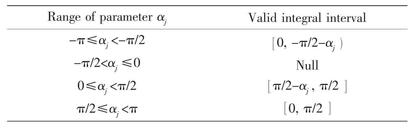
Tab.1 List of the valid integral interval

3.2 Numerical integration

The high and changeable oscillating frequency of integrand exerts great difficulty on the numerical integration.Conventional methods are so hard to get the integral results quickly that sometimes may fail with not converging integration.In view of the above-mentioned behaviors,the numerical calculation can be carried out according to the following idea.The composite function k2wjfrom the exponential one can be defined as an intermediate variable.By mathematical transformation,the integrand of far-field wave component is converted to the production form of a complex function and an exponential function and the original integral is reconstructed into that about the intermediate variable.In each micro element,the complex function can be approached by a linear function.So the overall integral is the numerical summation of total amounts in every element.The integration method above can transform the element discrete of high oscillating integrand into the numerical discrete of a complex function with no vibrations,which may reduce the difficulty and cost effectively.

By performing a mathematical transformation as κj=k2wj,the far-field wave component can be rewritten as follows:

where hjis a complex function whose representation is presented as follows:

where parameters c and d are easy to obtain as

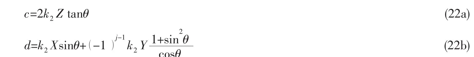
The complex functions,corresponding to the partial derivatives in three dictions are-ik2cosθhj,i（-1）j-1k2sinθhjand-k2hj,which can be expressed succinctly as hxj,hyjand hzj,respectively.If the valid integral interval is[θ1,θm]in Eq.(14b),the integral variable can be dispersed into θ1,θ2,θ3,…,θm,corresponding to the scattered points as κj1,κj2,κj3,…,κjmfor the new variable in Eq.(20).For the integrand of far-field wave component,the complex function hjcan be approximated by a linear function with one variable between two adjoining points as κjnand κjn+1for 1≤n≤m-1.Consequently,the integral Snin micro interval [θn,θn+1]can be presented as follows:

In the valid integral range,the three partial derivatives of far-field component can be numerically treated by a similar way.

4 Stable implementations for far-field wave component

In section 3.2,the key is the calculation of the complex function and its partial derivatives whose precision shows significant impact on the numerical result for far-field component.Below are the specific implementations to ensure the integral accuracy and stability for the endpoints and fake singularity.

4.1 Finite truncation of integral interval

When θ goes to π/2,complex functions hjand hxjpossess the limits but hyjand hzjdo not.So θ=π/2 is the infinite discontinuity for hyjand hzj.From the functional behaviors of far-field component,the oscillating amplitude tends to zero if θ→π/2.It is certain that an appropriate cut-off point θccan be found at θ=π/2 nearby to guarantee that the integration in[θc,π/2]is less than an integral error like e.For hyjand hzj,the infinite singularity can be eliminated by neglecting the integral result in the small interval of [θc,π/2].From the representations in Eq.(16),the magnitudes of y-and z-partial derivatives are roughly equal and larger than that of the integrand and x-partial derivative forthe far-field component.Here,the cut-off point θcis determined by the y-partial derivative.For the integrand,x-and z-partial derivatives,the absolute value of truncation error in[θc,π/2]is certainly lower than the integral error e.The representation of θccan be deduced as follows.

And e is taken as 10-5in general to ensure that the truncation error is lesser than 10-5.However,the integral error must be at a lower level of one magnitude thanif both the source and field points are adjacent to the free surface.

4.2 Effective combination of integral methods

In the particular condition of Y=0,θ=0 is the infinite singularity for complex functions as hj,hxjand hzj.If the spatial location of the source and field points is known,the oscillating frequency of the integrand largely depends upon the value of wave number k2for the far-field wave component.An obvious property is that k2is varying slowly and its value is keeping at a low magnitude in the neighboring interval of θ=0,where the oscillating frequency is relatively small correspondingly.It is important to note that θ=0 is not the singularity by θ-variable integration.An effective treatment is the partition processing for integral interval[0,π/]2.In the segmented interval near θ=0,the numerical calculation is performed by the θ-variable integration and implemented by the adaptive Simpson algorithm.In the remaining interval with the valid integral interval taken into account,the integration is carried out by the representation about κj.According to the actual need,the interval near θ=0 can be taken as[0,π/1]0,in which the integrand does not oscillate even one period in most cases.

4.3 Discrimination and solution of fake singularity

If Y≠0 but d=0,the complex function fluctuates strongly and even seems to appear the singularity character near the parameter θf,which is the root of Eq.(22b).In Ref.[23],this phenomenon is defined as fake singularity and must be paid great attention.Fig.3 gives the real and imaginary parts of complex function h1in the condition of X=-60,Y=20,Z=-0.05 and U=5 m/s.The scope denoted with dashed box is where h1changes dramatically.In order to ensure the accuracy and efficiency of numerical integration,the fake singularity must be taken into account for the discrete distribution of integral interval.

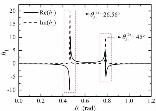
Fig.3 Fake singularity of the complex function

By the Eq.(22b),d=0 can be equivalent to a nonlinear equation as follows:

Apparently,the equation above is always true for X=0 and Y=0.Under such circumstance,the oscillating frequency is equal to zero by θ-variable integration and numerical integration is out of difficulty here.In order to discuss the condition that X and Y are not both zero or not zero at the same time,a transformation is introduced as b=-1/cosθ and b∈ （-∞,-1].So the Eq.(25)can be simplified as an equivalent equation about X,Y,and b.

For the equation above with j=1,there is no root if X=0 but Y≠0.However,b=-1 is the only one root for X≠0 and Y=0,and the root of original equation is θ=0 correspondingly.When X and Y are not both zero,Eq.(26)can be further transformed into that

According to the value range of b,X and Y,it is easy to deduce that 0＜-Y/X≤Therefore,only X and Y are contrary signs can the equation possess root(s).If X＜0 and Y＞0,the valid integral interval is not null from Tab.1 and the fake singularity may be present.Here,the Eq.(27)is rewritten as follows:

in which a=Y2/X2.The equation above can be regarded as a quadratic equation in one unknown of b2and the necessary condition is a≤1/8 for the existence of root.Correspondingly,X and Y must satisfy the condition of-Y/X≤.In physics,-Y/X implicates a tangent value of the angle θp,which is between the projected horizontal distance of source point from field point and the opposite speed direction of the advancing source.It is easy to figure out that θp≤tan-1）=19.47°and 19.47°is exactly the cusp angle of Kelvin wave[27].If j=1,the existing condition of fake singularity is therefore that the field point is just in the propagating region of Kelvin wave produced by the advancing source and Y＞0.At this point,the roots of Eq.(28)are as follows:

If a＜1/8,there are two different real roots for Eq.(25),which implicates that the fake singularities of complex function h1areThe root number will reduce from two to only one for a=1/8 and this real root is that θh1=35.26°.Similarly known,the fake singularity is being if the field point is exactly in the propagating region of Kelvin wave and Y＜0 for j=2.

In terms of the condition of Fig.3,the angle θpequals to 18.43°,which is smaller than 19.47°.So it can be discriminated that the number of fake singularity is two for the complex function h1.By the extract equation as Eq.(29),are equal to 26.56°and 45°,respectively,which is consistent with that illustrated in Fig.3.During the process of numerical integration,the fake singularity can be fast judged by the relative position of the field point and source point and evaluated by the extract equation directly.Then the local refinement is implemented numerically to increase the integral precision.

5 Numerical validation and analysis

To validate the accuracy and feasibility of integration methods above,Fig.4 shows the calculation results of the translating source Green function and its z-partial derivative,which are compared with those from Ref.[28].In the numerical example,the source point is located at （0,0,-）

1and moving with the speed U=2 m/s towards the positive direction of x-axis.The field point is at a ray of the undisturbed water plane and the included angle is tan-1（0. ）5between the ray and x-axis.As seen from Fig.4,the present results are almost consistent with the calculations by Inglis and Price,which indicates that the integral algorithm proposed is verified and applied to the numerical calculation for the steady translating source Green function and its partial derivatives.

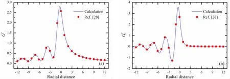
Fig.4 Behaviors of the Green function and its z-partial derivative for the source point located at （0,0,-）1

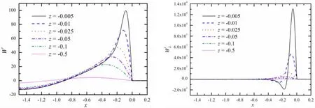
Fig.5 Behaviors of the wave component and its z partial derivative for the source point located at （0,0,）0

By the characteristics of exponential integral function,the value of near-field flow disturbance decays quickly as the increasing distance between the field point and the source point.However,the integrand of far-field wave component is an oscillatory function and this oscillating property is physically bound up with the wave-making profile on the free surface.In other words,the far-field wave component is the propagation mode of the Green function and describes the steady wave propagating outwards.Fig.5 illustrates how the far-field component and its z-partial derivative change when the vertical coordinate of field point is relatively small.Here,the field point is within the xoz plane and the source point is set at （0,0,）0 with the same speed as Fig.4.From the Fig.5,the wave component will fluctuate if x or z tends towards 0,which puts more demands on the numerical stability of integral methods when R or z-ζ is at small quantity.And the condition above is corresponding to the line integration in the boundary integral equation for the most part.In addition,the numerical results reveal that the integral value is zero if x＞0,which fits well with the actual fact that no waves exist ahead of the advancing source.

6 Conclusions

(1)Present work is started with the double-integral form of 3-D translating-pulsating source Green function in frequency domain.By the value property of zero advancing speed and nonzero oscillating frequency for the translating source,the integral term included with k1can be neglected.And it is testified that the 3-D translating source Green function is degraded into a real function based on the complex and conjugate attributes of the terms with k2.

(2)By performing linear transformation,a new mathematical representation of translating source is obtained with the summation of near-field flow disturbance,far-field wave component,Rankine source and its mirror of undisturbed water plane.The integral form is relatively simple with a single integral and the integral interval is limited to[0,π/]2.

(3)There is out of infinite singularity for the near-field flow disturbance in the deduced representation of Green function.The main integral difficulty lies in the peak character at the jump discontinuity of real part of ln （ wj）.To avoid the waste of computational resource and take the numerical efficiency into account,the variable step-length adaptive Simpson integral method is employed which can balance the contribution of the entire result from the integral error in each micro subinterval.

(4)For the far-field wave component,the composite function in the exponential function is defined as an intermediate variable and the integrand is then presented with the production of a complex function and an exponential function by mathematical transformation.This integral method can transform the element discrete of high oscillating integrand into the numerical discrete of a complex function with no fluctuation.The fake singularity of complex function is related to the propagating region of Kelvin wave.Only when the field point is within the wave scope of the translating source and notations of X and Y are contrary can the fake singularity show.The maximum number of fake singularity is two and the singular point can be fast resolved by extract equation to implement the local refinement in the integral interval.

Numerical validation and results show that the proposed method and program are reliable with high precision and high efficiency and applied to the calculations of translating source Green function and its partial derivatives for any field point and source point with different advancing speed.It is expected to numerical calculations of the wave-making resistance and steady wave profile for ships and marine structures.