Mohamed M. Kamra , Nik Mohd , Cheng Liu , Makoto Sueyoshi , Changhong Hu

1. Interdisciplinary Graduate School of Engineering Sciences, Kyushu University, Kasuga, Fukuoka, Japan

2. Research Institute for Applied Mechanics, Kyushu University, Kasuga, Fukuoka, Japan

Abstract: The three-dimensionality extent of the dam break flow over a vertical wall is investigated numerically and experimentally in this paper. The numerical method is based on Reynolds averaged Navier-Stokes (RANS) equation that describes the three-dimensional incompressible turbulent flow. The free surface is captured by using the unstructured multi-dimensional interface capturing(UMTHINC) scheme. The equations are discretized on 2-D and 3-D unstructured grids using finite volume method. The numerical simulations are compared with newly conducted experiment with emphasis on the effect of three-dimensionality on both free surface and impact pressure. The comparison between the numerical and experimental results shows good agreement. Furthermore, the results also show that 3-D motion of the flow originates at the moment of impact at the lower corners of the impact wall and propagates to the inner region as time advances. The origin of the three-dimensionality is found to be the turbulence development as well as the relative velocity between the side wall region and the inner region of the wave front at the moment of impact.

Key words: Water impact, dam break flow, UMTHINC scheme, three-dimensionality

Introduction

Dam break flows refer to the collapse of water columns, initially at rest due to the removal of a gate or flap, under the influence of gravity. Despite its simplicity, these gravity-driven flows have been studied theoretically, numerically and experimentally for many years either as means for the validation of CFD codes or simply to understand more complex related flows such as wave loads on coastal structures,sloshing loads in tanks and green water loads on ships.

For many years, several experimental studies were carried out on dam break flows. Most of them aimed to compare the shape of the free surface and wave front as well as the time evolution of the wave front and its velocity[1-4]. Other experiments aimed to study the water impact loads on ships and offshore structures as well as provide more quantitative data about the flow such as water level elevation, pressure impulse and impacting force[5-10]. In the numerical modeling of dam break flows, some of the relevant aspects of the flow physics were either not modeled or under-estimated in the numerical simulations. Therefore, some differences are observed when comparing with experimental data. These important physical aspects include but not limited to:

(1) Wall/hydraulic resistance increase due to the turbulence developing in the flow. This aspect was investigated by Park et al.[11]using volume of fluid(VOF) algorithm coupled with Reynolds averaged Navier-Stokes (RANS) equations. The effect of the initial value of turbulence intensity as well as the surface roughness effect on the water front shape and speed, water elevations and pressure impulse was examined. The authors argued that a higher turbulence intensity showed considerable improvement in the accuracy of the computed pressure and wave front speed when compared to experimental data[10].

(2) Gate obstruction: Despite the fact that nearly all dam break experiments satisfy the condition of sudden gate removal as prescribed by Lauber and Hager[2], some differences still exist between the numerical and experimental data. Sueyoshi and Hu[12]investigated the gate effect using the moving particle semi-implicit method (MPS). The authors used solid particle to model the gate motion and reported better agreement with respect to the wave front propagation as well as the water elevations. Further numerical investigations were performed by Ye et al.[13]who demonstrated that the gate effect in obstructing the collapse of the water column and changing the shape of free surface and wave front still exists regardless of the gate removal time. The authors studied the effect of different gate motions on the pressure impulse,wave front speed, and free surface shape. The authors concluded that the gate obstruction causes the wave front to be faster at first but slower as time passes.Such behavior would account for the lag in the impact time in some numerical results. The gate motion may also affect the impact pressure producing higher pressure magnitude when compared with the no-gate case.

(3) Three-dimensionality: The two studies mentioned previously are both based on 2-D numerical results. In fact, to the best of the authorsʼ knowledge there is only one experimental study by Lobovsky et al.[9]which briefly mentions the extent of threedimensionality in dam break flows. The article compared the time history of two pressure sensors on the same height and reported similar time histories with some differences in terms of the peak pressure value and time of impact.

In this article, further numerical and experimental investigation into the extent of three-dimensionality in dam break flows is carried out. Numerical simulations are performed using a newly developed Reynolds averaged incompressible Navier-Stokes equations solver coupled with the volume of fluid (VOF)algorithm. Interface capturing is performed using the unstructured multi-dimensional tangent hyperbolic interface capturing (UMTHINC) sche- me[14-18]. In this work, the gate motion effect is not taken into account in the numerical simulations. An experiment was performed in the Research Institute of Applied Mechanics at Kyushu University in order to validate our numerical code. The experiment utilizes high-resolution imaging and six pressure sensors placed on the impact plate. The extent of threedimensionality is investigated by comparing the wave front evolution, free surface profiles as well as the pressure time histories. The effect of the tank width on the extent of three-dimensionality is reported as well.

1. Numerical method

1.1 Governing equations

The 3-D RANS equation for the present incompressible two-phase flow simulations is given by

where ρ is the density,eμis the effective viscosity defined as the sum of the turbulent eddy viscositytμand molecular dynamic viscosity μ, t is time, V is the velocity vector, and p is the static pressure.The effect of surface tension is neglected due to its limited effect in body force dominated flows. To ensure balance for the gravity force, a working pressure variable is defined[19]as p=P-ρg· x where p is the working pressure variable, g is gravity and x is the position vector. Therefore, the momentum equation can re-written as

1.2 Turbulence modeling

Turbulence modeling is handled by the two equation standard k-ε model[20]. To avoid mesh refinement in the viscous-sublayer, standard wall function is employed[20-22]. In the standard k-ε model the turbulent eddy viscositytμ is defined as

where Cμis a dimensionless constant with a typical value of 0.09, k is the kinetic energy of turbulence and ε is the turbulence dissipation rate of turbulence kinetic energy. The transport equations for the k-ε two equation model are given by

where σk=1.0, σε=1.3, Cε1=1.44 and Cε2=1.92. In this work, the wall surface is assumed smooth thus surface roughness is neglected. The initial values for k and ε are set as discussed in Ref. [11].

1.3 Two-phase flow modeling

The interface between the two phases (water and air) is identified using the volume fraction α which is defined as the volume average of the indicator function over the computational cell.

where ρ1,2and μ1,2are the density and viscosity properties of water and air respectively. The time evolution of the volume fraction equation is governed by the following advection equation.

In the UMTHINC method, the interface jump is defined as a smoothed piecewise hyperbolic tangent profile[14], so the indicator function is approximated as

where β is the sharpness parameter which controls how steep (thin) the interface region between the two fluids is, and the interface surface equation is defined by(x)+d=0where d is a coefficient which represents the interface position in the computational cell and P(x) is a second order polynomial with coefficients based on the interface geometric characteristics such as the unit normal vector n =(nx, ny,nz) and curvature matrix Ixyzof the interface.

In this work, only linear interface reconstruction is considered thus P(x) is reduced to a linear function dependent on the interface normals. Reconstruction is made for interface cells that is identified by∈＜α＜（1.0- ∈） being ∈ set to 10−8in this paper.The reader is referred to articles[15-18]for further details.

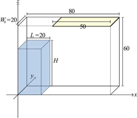
Fig. 1(a) (Color online) Schematic drawing of the problem of dam-break against a vertical wall (all dimensions are in cm)

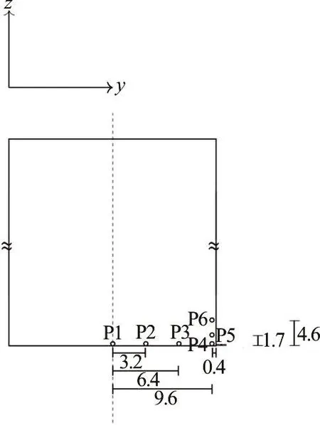
Fig. 1(b) Sensor placement on the right vertical wall (all dimensions are in cm)

Table 1 Mesh spacings of the three grid adopted in the mesh independence test

1.4 Numerical implementation

In this work, the 3-D incompressible turbulent flow is solved using the cell-centered finite volume method based on second order discretization in space as discussed in Refs. [21-22]. For all simulations conducted in this work both 2-D and 3-D, a set of mixed elements unstructured grids are employed. All grids consist of orthogonal quadrilateral/hexahedral cells near the boundaries for accurate boundary treatment and triangles/prism cells elsewhere.

Fig. 2 (Color o nline) Mesh independence test, the force coefficient isdefinedas with

The pressure-implicit with splitting of operators(PISO) non-iterative time advancement method[19,23]is employed with 4 neighbor correction during each time step to ensure that both the continuity and momentum equations are sufficiently satisfied. First order time implicit scheme was applied for the time discretization of the momentum equation. Adaptive time stepping was employed based on the convective time step restriction due to the local Courant number.The second order total variation diminishing (TVD)limited linear upwind scheme was applied for the convection term with the Van-Leer limiter[21,24-25].The cell-based Green-Gauss method was used to compute the velocity and pressure gradients.

Fig. 3 (Color online) Time evolutions of the wave front toe position (a) and velocity (b) compared with literature

Table 2 The non-dimensional average velocity v/ of the wave front toe for t*＞1

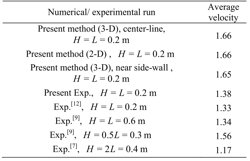
Table 2 The non-dimensional average velocity v/ of the wave front toe for t*＞1

?

The finite volume formulation of the UMTHINC method is written as

where j is thethj face of celliΩ,ijα is the face value of the volume fraction,is the face area,and vnijis the normal velocity on the face.

(1) The numerical procedure used to implement UMTHINC, in this work, can be summarized in the following steps:

The calculation of the interface unit normal vector n =(nx, ny, nz)at the cell center

(2) Calculation of the unknown d such that Eq.(7) is satisfied.

(3) Calculation of the face value of the volume fractionijα.

(4) Advancing the volume fraction equation in time.

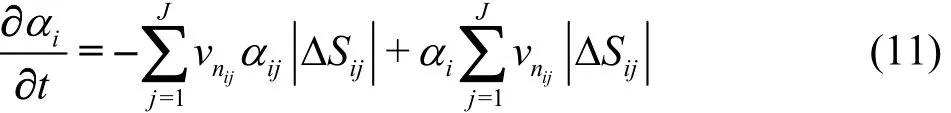
In this work, the unit interface normals are computedusingthenode-averaged-gauss(NAG)method[26]. The methods used to compute the unknown d and face value of the volume fraction ijα are explained, in detail, in Refs. [15-18]. The explicit 3 stage low storage TVD. Runge-Kutta scheme[27]is used to advance the discretized volume fraction equation (Eq. (11)) in time.

2. Results and discussions

The initial setup for the 3-D dam break flow against a vertical wall is depicted in Fig. 1. The water column is confined (trapped) by the bottom wall, the moving vertical gate and three vertical walls. Once the gate is removed, the water column collapses under the influence of gravity (g =9.81m2/s)and the water flows on the dry horizontal bed. The dimensions of the tank are based on an experiment conducted in the Research Institute of Applied Mechanics, Kyushu University.

The dimensions and specifications of the dambreak experiment is clearly shown in Fig. 1. The water column height is H=0.2 m and the length and width are L=W0=0.2 m . Six pressu re senso rs are mounted on the right vertical wall. Thesensorshave 0.8×10-2m diameter and are mounted as illustrated in Fig. 1(a). The sensor placement is intended to explore the extent of three-dimensionality and the side wall effect. The tank top is closed by cap extending 0.5 m from the right vertical wall.

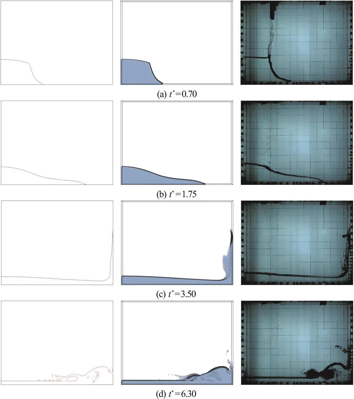
Fig. 4 (Color online) Comparison of the free surface profiles (front view) at selected time instances. The left: 2-D section at the domain center line(red: 3-D, blue: 2-D), middle: 3-D perspective front view, right: experiment perspective front view

Fig. 5 (Color online) Comparison of the free surface profiles (3-D iso-metric view) at selected time instances

In the numerical simulations, the density of water and air is set to 997 kg/m3and 1.185 kg/m3respectively,while the molecular viscosity is set to 0.0089 kg/(m·s)and 1.7894 × 10−5kg/(m·s) respectively.

Three 2-D grids were adopted to investigate mesh dependence of the numerical solution. The minimum and maximum mesh spacing for the three grids is provided in Table 1.

Figure 2 shows the wave front, free surface profile and forces over the impact wall solved on three different grids. The results of the fine and medium grids are fairly close while the coarse mesh shows considerable difference especially for the viscous shear force. Therefore, in the subsequent numerical computations both 2- D and 3-D, grids with minimum spacing of 0.5 mm and maximum spacing of 5.0 mm will be used.

Figure 3 shows the time history of the position and velocity of the wave front as compared with several recent experimental results. Some discrepancy is found between numerical and experimental data.These discrepancies can be attributed to the gate obstruction of the flow, which is not modeled in this work, as discussed in Refs. [12-13]. As the gate opens a strong water jet with high velocity emerges from the clearance under gate while the rest of the water column is still obstructed by the moving gate. Once the gate is fully open, the wave velocity decreases then starts to increase again in a steadily manner similar to the numerical simulation.

An interesting point is that in the absence of gate influence, the numerical results approach the theoretical value[28]in an asymptotic manner while the experimental data is trying to cross it. This point was also observed in the numerical solution of Ye et al.[13]when the gate effect was modeled in the simulation.This may be due to the added kinetic energy and vorticity to the free surface by the gate motion.

A quantitative analysis of the average velocity of the wave front after t*＞1 is given in Table 2. The discrepancy between the numerical and experimental data is caused by the same reasons mentioned previously. Additionally, Table 2, Fig. 3 show that the wave front velocity adjacent to the tank side-walls is less than central line by no more than 1%. This indicates the weak extent of three-dimensionality before the wave impacts the right vertical wall.

Table 2 also indicate a close relation between the average non-dimensional wave front velocity v*and the ratio (H/ L). The relation implies that the wave front velocity is strongly dependent on the ratio(H/ L) and inversely proportional to its value.

The wave front position, for the numerical simulation as well as the present experiment, can be fitted into an algebraic equation using MATLAB in the following form

where t*is the non-dimensional time (t*=t)and the coefficients a0, a1and b0are given in Table 3.

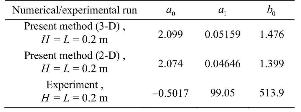
Table 3 Coefficients of the fitted equations for numerical and experimental data of the time history of the wave front position as in Fig. 3

An expression for the wave front velocity can be obtained by differentiation of Eq. (2). In Table 3, the coefficients of the fitted equations of the 2-D and 3-D numerical results are fairly similar however the experimentʼs coefficients are completely different.

Figures 4, 5 show the evolution of the free surface from two different view angles at selected time instants. Pictures of the free surface of the experiment is also presented for both view angles at the same time instants for comparison.

Owing to the effect of the gate, a splash of water is observed in the initial stages as shown by experimental pictures. Additionally, there are some differences in the free surface profile due to obstruction of the gate and the free surface disturbance from the falling drops. However, the numerical simulation agrees very well with experimental pictures. It is observed that until the wave front impacts against vertical wall, the free surface is 2-D in the x- z plane and the wave front is nearly straight with some curvature near the side walls due to the no-slip wall boundary.

Figure 4 shows contour line (α=0.5) for the 2-D case and the center-line section of the 3-D case. It is observed that contour lines nearly coincide until the wave impacts the vertical and the free surface collapses on itself to become fully 3-D. Prior to impact, the velocity near the side-wall is slower than the center-line area owing to the no-slip boundary.However, after impact, the sides of the wave front become faster than the central area. Additionally, the side walls show some wetting near impact zone which keeps increasing until the wave runs up the vertical wall. This is observed in both experiment and simulations as shown by Figs. 4, 5.

Fig. 6 (Color online) Velocity vectors in the bottom right corner area of the impacted wall at the moment of impact. The figure is a magnified bottom view of the corner where the blue region represents water and the white represents air

This can be explained by examining the flow behavior in the corners at the moment of impact as shown in Fig. 6. By virtue of the boundary layer at the side walls, a vortex-like flow occurs when the flow impacts the wall[9].

Consequently, the water moves from the center to sides which would result in the wetting of the side walls and the loss of momentum from the inner region to sides. This would also account for the irregular shape of the wave front in Figs. 5(d)-5(f) as the water climbs the wall.

Fig. 7 (Color online) Time histories of the pressure at the vertical wall

The comparison between the computed pressure history and experimental data, at the six prescribed location depicted in Fig. 1, is given in Fig. 7. The 2-D result is compared with the three dimensional results and experimental data for sensors P1 -P4. Generally,the numerical simulation agrees well with experimental data but the numerical simulation seems to under-estimate the value of the first and second pressure peak. This could be the result of excessive diffusion generated by the two-equation k-ε model which could be mitigated by using a higher order turbulence closure model[11]. It can also be observed that a sudden pressure drop occurs for sensors P4 -P6 in the interval 3＜t*＜4 which may be the result of small air-pocket or bubbles.

Figure 7(a) shows very good agreement with experiment and the 2-D result seems to generally over-estimate the pressure when compared with 3-D numerical results and experimental data. As we move away from the center-line the difference between the 2-D and 3-D results increases in both magnitude and phase as shown by Figs. 7(a)-7(d). Figures 7(d)-7(f)show the pressure variation with height adjacent the side walls. The pressure experimental data shows an increase in the oscillatory behavior as the height increases. This may be attributed to either the pressure sensors ability to accurately detect such low pressures or simply the excessive bubble formation adjacent to the side wall after impact. As a result, the comparison with the experimental data deteriorates with height.

Fig. 8 (Color online) Pressure distributions in the transverse direction at the vertical wall for selected time instants

The pressure distribution in the transverse direction is given in Fig. 8 at selected time instants. At the early stages just after impact, the pressure variation seems localized to side wall areas. As time advances the pressure variation extends to the inner part of the domain. It is also observed that the magnitude of the transverse pressure variation decreases as we move away from the bottom wall. This would suggest that source of three-dimensionality is the 3-D vortices localized at the lower corners of the impact wall.

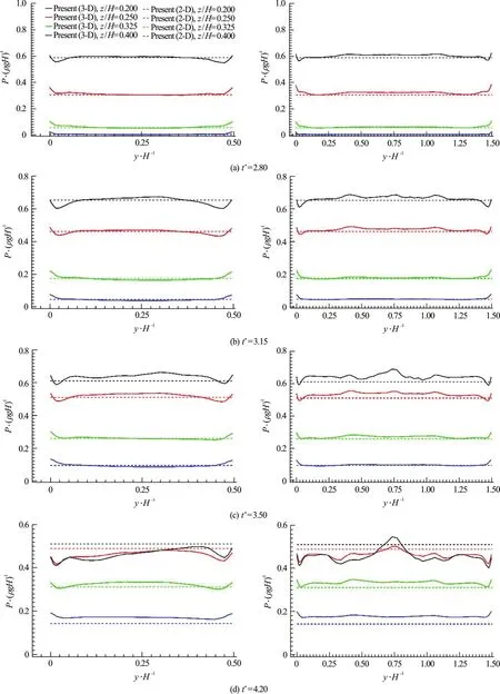
Fig. 9 (Color online) Effect of tank widths on the pressure distributions in the transverse direction at the vertical wall with left(W=0.1m) and right (W=0.3m)

The effect of the tank width is explored by running numerical simulations for two additional tank widths of 0.1 m and 0.3 m. In Fig. 9, the pressure variation in the transverse direction is compared with the existing case in Fig. 8. For all tank widths, the threedimensionality originate from the side walls and advances across the transverse direct as time progresses. Larger tank width affects the pressure distribution in the transverse direction and results in localized higher pressure regions towards the center.However, smaller tank width gives closer comparison to the 2-D solution with localized discrepancy near the side walls. As time advances, the semi-symmetric pressure distribution breaks much faster than the other two cases due to the interaction of the side-wall vortices.

3. Conclusions

The extent and cause of three-dimensionality in the dam break flow against a vertical wall was investigated in this work. 2-D and 3-D numerical simulations have been conducted and compared with a newly developed experiment.

The comparisons were focused on the free surface profiles and impact pressure history. The results show that the flow remains 2-D until the moment of impact. The free surface profile at midsection of the 3-D simulation is comparable to the 2-D simulation until free surface collapse on itself after impact. The 2-D simulations tend to over-estimate the pressure distribution when compared with the 3-D simulations and experiments.

After the impact, the three-dimensionality originates at the sidewalls and propagates to the inner regions of the domain as time passes. The source of three-dimensionality is found to be the turbulence development as well as the relative velocity between the side wall region and the inner region of the wave front at the moment of impact.