Giorgio Contento, Guido Lupieri, Thomas Puzzer

Department of Engineering and Architecture, University of Trieste, Trieste, Italy

Abstract: The interaction of regular quasi-monochromatic waves with a weakly submerged rectangular shelf is studied by means of CFD simulations. The fundamental incident wave frequency is kept constant for the full set of simulated cases, while the incident wave amplitude is made increase progressively, so that the interaction with the shelf is dominated by almost inviscid non-linear flow for the smallest and by breaking for the highest incident waves. A parameter identification (PI) procedure is used to adapt a reduced model to the highly resolved time-space matrix of wave elevations obtained from the numerical simulations, on the weather and lee side respectively. In particular the wave number and the frequency of the component waves in the reduced model are left uncoupled, thus computed by the PI independently. The comparison of simulated data with experiments generally shows a very good agreement.Free/locked, incident/reflected, first/higher order wave components are quantified accurately by the PI and the energy transfer to super-harmonics is clearly evidenced. Moreover the results of the PI show clearly a very large increase in the phase speed of the higher order free waves on the lee side of the shelf, with increasing deviation from the linear behavior with increasing incident wave amplitude.

Key words: Nonlinear wave transformation, submerged shelf, wave breaking, coupled space-time domain analysis, reduced model,parameter identification

Introduction

Wave transformation past submerged or surface piercing obstacles and wave-induced loads on the obstacle are subjects of great interest in free surface hydrodynamics. It is related to the protection of near shore structures, to harbor design, etc. The efforts done to understand the fundamentals of this phenomenon or of closely related phenomena including both experimental and theoretical investigations, the adoption of simplified geometries, analytical or computational methods, viscous or inviscid flow simulations,Bousinnesq type models, turbulence modeling and wave breaking. The literature on these subjects is extremely wide.

Wave transmission and reflection coefficients by a shelf have been investigated numerically in an early work by Newman[1]who adopted an approximate analysis, considering separately the effects of diffraction at the ends of an obstacle, and showing the effect induced by the obstacle length. The propagation of surface gravity waves over a bar has been studied experimentally and by a theoretical model also by Rey et al. (1992). In the experiments, in order to visualize the flow path lines, the authors injected dye in the fluid and observed the vorticity structures produced at the corners of the bar, using a camera through the channel sidewalls. Grue[2]studied the characteristics of waves passing over a very shallow rectangular shelf. Laboratory data and numerical predictions, obtained by a nonlinear solution of the inviscid irrotational flow,showed the strong transfer of energy to super-harmonics. The results on the lee side were presented in space-averaged form, but still distinguishing clearly between free and bound waves. Even though the steepness of the incident waves was very small, the theoretical predictions of the inviscid model were limited by wave breaking occurring in the very shallow water above the shelf. Ohyama and Nadaoka[3]considered the decomposition of a wave train passing over a submerged shelf in the absence of breaking events. The investigation was conducted with a fully nonlinear inviscid flow model. They showed that the distribution of the amplitude of the second and third harmonics along the domain exhibits spatial modulation over the step because of resonant interactions between free and bound waves. This phenomenon was said to trigger the generation of higher harmonics that propagate from the obstacle on the lee side. In a laboratory experiment, Ting and Kim (1994) computed the energy bounded in the vortices generated at the obstacle by measuring the velocity field with the goal to estimate the energy loss in the surface wave train.Ohyama et al. (1995) studied the applicability of three different wave propagation models in nonlinear and dispersive wave fields: a fully non-linear potential theory, a Stokes second order and a Boussinesq type theory. Wave evolution during the passage over a submerged shelf was examined with the following conclusions: the second order theory (Stokes) cannot describe energy transfer among harmonic components,the Boussinesq model is more accurate but tends to overestimate the amplitude of some super-harmonics,the fully non-linear model is closer to experiments.Losada et al (1996) studied the linear interaction of regular waves with a permeable breakwater within the inviscid flow approximation. Hsu et al.[4]studied the viscous effects in the flow induced by waves propagating over a double rectangular breakwater without breaking, with obstacle height of the order of half water depth in the far field. The generation of higher harmonics by non-breaking surface waves traveling over a submerged obstacle was examined experimentally by Ting et al.[5]in a wave flume. They found that super-harmonic waves are generated in correspondence to the obstacle, they propagate on the lee side and their order increases with non linearity of the wave defined in terms of Ursell number. Sue et al.[6]investigated numerically the interaction of viscous progressive waves with a submerged rectangular obstacle by solving the RANS equations within the k-ε turbulence model. They showed the results related to free surface elevation and vorticity patterns.They considered the ratio of wave height to water depth to characterize the nonlinearity of incoming waves and to reveal that highly nonlinear waves induce stronger vortices around a submerged obstacle. Another relevant ratio is the wave height to obstacle width (size effect). It was observed that the vortex motion around the obstacle is enhanced as the length of the submerged obstacle decreases. Johnson[7]studied the behavior of waves and current around submerged breakwaters using both a phase-averaged method of the MIKE family of the Danish Hydraulic Institute (DHI) and a phase resolving method based on the Boussinesq type model. They found that wave height compares well to measurement if the wave breaking sub-model is properly tuned for dissipation. Johnson et al.[8]studied a 3-D wave transformation induced by two submerged breakwaters parallel to the crest lines, in a harbor entrance like pattern. The study was conducted both experimentally and numerically using the commercial software MIKE 21 PMS by DHI, with a special treatment of wave breaking. Lu et al.[9]investigated experimentally and numerically with a RANS/VOF model two-dimensional overtopping against a seawall in regular waves. The numerical implementation included very efficient absorbing zones at the weather and lee side of the obstacle. Christou et al.[10]studied the nonlinear inviscid interaction between regular waves and a rectangular breakwater, without breaking,with obstacle height of the order of half water depth in the far field, varying the breakwater length and comparing the result with experimental data. Guo et al.[11]investigated numerically with a RANS/VOF model regular waves overtopping flows induced by a smooth trapezoidal sea dike. A large amount of work has been successfully devoted to the efficiency and accuracy of wave generation and absorption in strongly nonlinear waves. In the same context, a large campaign of model calibration tests has been undertaken in order to achieve a quasi-optimal performance of the turbulence model.

The present work tackles the problem of a 2-D regular quasi-monochromatic wave train traveling over a submerged rectangular shelf, mounted over a horizontal flat impermeable bottom. In particular the case study regards a very shallow water condition over the shelf so that wave breaking and strong nonlinear effects are expected even in small amplitude incident waves. The diffraction regime holds. The study is conducted via CFD numerical simulations and analysis of the results via reduced model. Two-phase flow Navier-Stokes equations are solved by a Finite Volume technique and Volume of Fluid treatment of the free surface interface[12]. In the present study, reference experimental data are those presented by Grue[2]. In particular the simulations have been conducted assuming the same physical set-up of the experimental basin, i.e., a piston-type wavemaker at one end of the basin and an absorbing zone at the opposite end. The simulations are meant at the reproduction of the experiments conducted in a narrow closed basin, rather than reproducing open water data. The lack of absorbing devices at the weather side of the shelf implies that the analysis of the results must be conducted consistently with the experiments and with accurate data windowing.

The key point of the work stands in the analysis of the wave train on the lee side and specifically in the energy transfer to free and/or locked waves and mostly in the strong nonlinear features of phase speed of these components in the near field.

As expected, the results in the frequency domain at given independent stations on the lee side reveal a large transfer of energy to higher harmonics, up to the fourth, with a strong nonlinear growth of the nondimensional amplitude with the incident wave height and with a progressive decrease after breaking.

However, the most relevant part of the study concerns the longitudinal properties of the transmitted waves, wave celerity in particular. A coupled spacetime analysis of the wave elevation at a very large number of stations-instants shows that free waves, first and higher harmonics, travel largely faster than linear waves, with increasing deviation from linear dispersion with increasing incident wave amplitude.

The analysis of this phenomenon is conducted using a reduced model fitted to the large matrix of space-time free surface elevations gathered from the numerical simulations. The proposed reduced model is given by the superposition of free, locked and reflected harmonic waves, whose amplitudes, phases and mostly wavenumbers are parameters left free in the fitting.These waves do not necessarily obey the linear dispersion. A Parameter Identification is applied to the proposed reduced model to compute the entire set of unknown free parameters.

1. Problem formulation

1.1 Physics

The physical problem consists of regular ideally monochromatic unidirectional gravity waves with length λ, angular frequency ω and amplitude a=H/2 that travel past a submerged obstacle. Here the obstacle is a rectangular shelf with small-radius rounded corners. The gap h between the upper part of the shelf and the free surface in still water condition makes the shelf a shallow water region whereas in the rest of the domain the water depth D can be considered deep for the wavelengths in use. The problem is assumed two-dimensional and it is studied in a closed basin, with a piston-type wavemaker and an absorbing beach at the opposite end.

A schematic representation of the problem is given in Fig. 1. A Cartesian frame of reference O( x, y) is here used with x-axis placed at the still free surface, in the direction of wave propagation, and the y-axis is upwardly oriented. The origin O is placed in correspondence to the average position of the piston-wavemaker.

The longitudinal L and vertical B extensions of the shelf are such that, compared to the incident wavelength λ, the diffraction regime holds (λ/L≈3,λ/B≈4). The maximum incident wave steepness here considered H/λ is very small, approximately 1/80 and the incident wave train can be assumed quasi-monochromatic.

In particular the problem here analyzed refers to one of the experiments of Grue[2], where L=0.5 m B=0.4125 m, D=0.45 m , h =0.0375 m and f=ω/2π=0.95Hz so that, in linear dispersion approximation, the wave length is λ=1.59 m . The length of the basin is 14.2 m and the front of the shelf is positioned at x=5.2 m from the average position of the piston-wavemaker. The simulations have been conducted for 7 different wave heights, keeping the wavemaker frequency constant, as reported in Table 1.

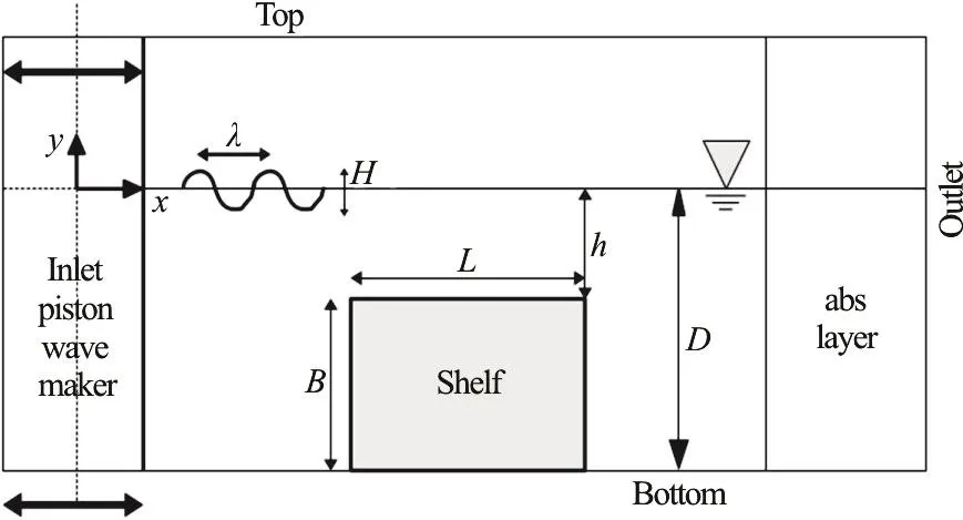
Fig. 1 Schematic representation of the problem

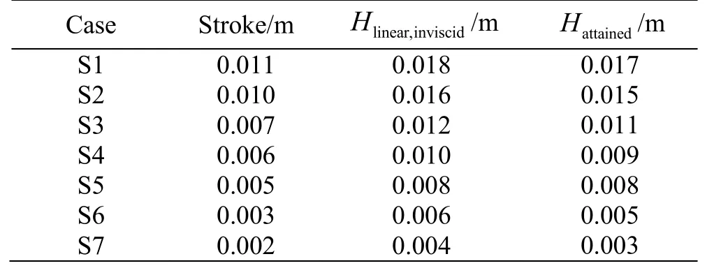
Table 1 Wa ve maker stroke for the simulated cases (piston),far field incident wave height from an inviscid linear model and wave height attained in the present simulations

The interaction between the incident wave and the shelf exhibits a variety of linear and non-linear features.

(1) Due to its vertical extension B compared to the water depth D (91.7%) and to the wavelength λ (26%), the shelf behaves like a potential wave reflector. Since the simulations reproduce the experimental set-up, no additional wave absorbers have been introduced on the weather side. In long time simulations the incident wave may become strongly polluted because of multiple reflections between the shelf and the wavemaker. From our results and from those of Grue[2], the reflection from the shelf has a basically linear nature and this makes its detection easier.

(2) On the lee side, super harmonic oscillations appear in the frequency domain at multiple frequencies of the incident wave n·ω, with =2,3,4,n…both for free “subscript f ” and locked “subscript l”waves, the latter being waves driven at the phase speed of the fundamental wave component n=1. If super-harmonic free waves have a small amplitude,the linear dispersion relation should hold, thus their wave length λf,nshould be

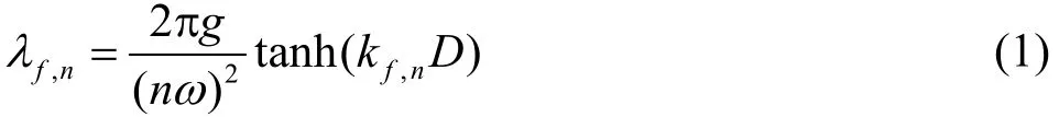
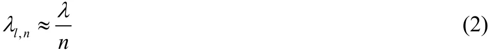
In Eq. (1) kf,nare the wave numbers of free waves.As for locked waves, their wavelength in deep water approximation λl,nbecomes

(3) Two non-linear effects are related to free waves specifically. (a) These waves may exhibit a strong nonlinear growth of their amplitude αf,nwith the increasing amplitude of the incident wave a. As a consequence, their own steepness may become very large and thus the linear dispersion Eq. (1) does not hold any longer. (b) On the lee side, the interaction with the shallow water zone may induce extremely large modifications of the wavelengths compared to those computed with linear dispersion (Eq. (1)). This nonlinear effect introduces some difficulties in the accurate decomposition of the transmitted wave train.This will be discussed thoroughly in Section “Model reduction” and Section “Parameter identification”.

(4) Last but not least, if the amplitude of the incoming wave train is made increase, the shape of the global wave starts exhibiting asymmetry at the shelf and breaking effects may become dominant. Spilling breakers appear first, so ideally without large bubble generation, then leading to plunging breakers, with overturning of the wave crest.

A final remark regards the wave train composition on the lee side. The fundamental and higher order free waves may be reflected from the beach, depending on the efficiency of the absorbing device, either physical or numerical. As anticipated above, in this work the reference experimental data are those of Grue[2]so that the entire set-up of the numerical simulations (domain size, wavemaker type, absorbing zones,··) has been tailored accordingly. A well-based data windowing has been adopted in the analysis of the results.

1.2 Model reduction

It may be useful to approximate the overall wave train in the basin in two branches, the weather and the lee side of the shelf respectively. In the case of regular incident waves generated at the wavemaker, the resulting wave train can be conveniently decomposed into component waves whose frequencies are ultra or sub-harmonics of the dominant frequency introduced at the wavemaker.

On the weather side, the wave elevation, at any time t and at any position x, from the wavemaker to the shelf, may be approximated as follows

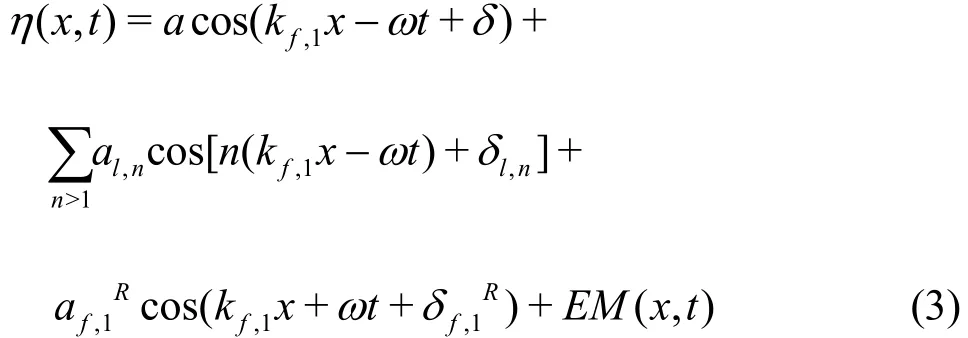
The first term on the RHS of Eq. (3) corresponds to the main incident free “f ” wave. The second term(sum) corresponds to locked “l” waves linked to the main incident wave. The third term corresponds to the wave reflected “R ” off of the shelf. EM( x, t) stands for possible evanescent modes close to the wave maker.is the amplitude of the wave reflected off of the shelf, at first order only. The amplitude of the reflected free waves, with n＞1, can be considered negligible so they are not introduced in Eq.(3). Finally, for symmetric wave profiles, δl,nshould be equal to δ. According to the results obtained during the present work, here δl,nis left as a free parameter and computed by the Parameter identification (PI) procedure (see related section).

Equation (3) assumes implicitly that there must be no multiple reflections between wavemaker and shelf. Indeed in the case of multiple reflections the first term in Eq. (3) is no longer representing the incident wave but the sum between incident and several reflected waves. As anticipated, this is consistent with the experiments and is discussed later on in Section “Data windowing”.

On the lee side, the wave elevation, at any time t and at any position x, may be approximated as follows

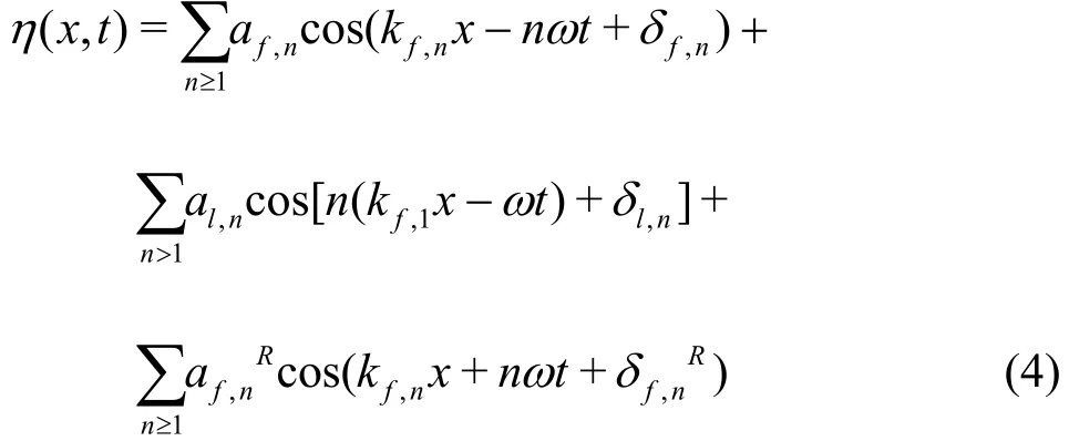
In Eq. (4), the first sum is over the transmitted free “f ” waves at any order, the second sum is over the locked “l” waves related to the main free wave whose wavenumber is kf,1, the third sum is over the free waves generated at the shelf and then potentially reflected “R ” off of the end of the domain. It is assumed that the locked waves reflected off of an efficient beach are reasonably small and thus negligible. Among others, this approximation has been used by Grue[3], and more recently by Andersen et al.[13], to split complex wave trains in components and then computing amplitudes and phases of reduced models via fitting techniques. Both Grue[2]and Andersen et al.[13]applied the linear dispersion relation between frequencies and wave numbers, at any order. This implies that any component wave was expected to behave linearly in terms of phase speed.In general this might not be the case. In our simulations we found that the transmitted free waves,mostly the higher harmonics, behave in a strongly nonlinear way in a space region of order some wavelengths of the dominant incident wave. For instance, the third harmonic free transmitted wave can be 20% faster than the corresponding linear wave of the same frequency. For this reason, in our analysis wave frequencies and wave numbers have been considered uncoupled. Specifically, a standard Fourier analysis at any x on a time record M/f long (i.e.,an integer number of dominant periods) shows clearly that the frequency content is confined to ultra and sub-harmonics only. These frequencies are introduced in Eq. (4) so that the set of unknowns becomes amplitudes, phases and wave numbers.

1.3 Parameter identification

From Eqs. (3), (4), for a given fixed position x,the representation of the wave elevation becomes a superposition of harmonics in which the amplitudes are a blending of free, locked and reflected waves,without any possibility of distinguishing between those components from a standard frequency domain analysis at a fixed station. On the contrary, using multiple stations x, it is possible to split the wave elevation in the components given by Eqs. (3), (4).Grue[2]has derived the amplitudes of the free transmitted waves (n≤3) using a technique based on the synchronous measurement of the wave elevation at two independent stations. Andersen et al.[13]have derived a procedure to distinguish between free,bound and reflected wave components with a four gauges technique. As discussed in Section “Model reduction”, both of them applied the linear dispersion relation between frequencies and wave numbers of the free waves at any order and for any incident wave steepness.

In this work a different strategy is applied. It uses the entire matrix of space time wave elevations obtained from the simulations. A least-square fitting of Eq. (4) is applied to this matrix in such a way that Eq. (4) becomes the best representation of the dataset in terms of least square error2χ of the wave elevation, anywhere and at any time. Thus, if ηSIMUL(xi, tj)is the wave elevation of the simulations at i=1,Nstationsand at j=1,Ntime, if ηMODEL(xi, tj)represents the wave elevation according to the reduced model given by Eqs. (3), (4), then Eq. (5) represents a quality index of the reduced model.

In this work we have extended the number of harmonics up to fourth order and the parameter identification has been extended to the free f,locked l and reflected R wave components. The least-square method, based on the Levenberg-Marquardt algorithm, allows to determine amplitude,phase and wavenumber of each component wave of the reduced model.

1.4 Data windowing

The accurate generation, propagation and absorption of waves in a closed basin, aimed at obtaining the target wave at the target stations, is a very well-known issue. It regards both experimental and numerical tests, among others Andersen et al.[13],Contento et al.[14], Higuera et al.[15], 27th ITTC–Specialist Committee on CFD in Marine Hydrodynamics[16], Swan[17]and Likke Andersen et al.[18].Controlled wavemaking and/or active absorption are almost mandatory techniques in long time experiments or simulations, in regular and irregular waves.Lu et al.[9]and Guo et al.[11]developed a 4 zones 2-D numerical wave tank in the RANS/VOF framework,where two distinct zones, on the weather and lee side of the body, act as absorbers of the undesired waves.The method is shown to extract waves reflected off of the body and reflected off of the end of the domain after the body quite well, still showing a small amplitude modulation for both pure progressive waves and pure standing waves without body.

Generally speaking, nonlinear effects show up in small percentages of the driving linear part of the phenomenon, thus even a small pollution of the data from wave reflections may lead to wrong interpretation of the real nonlinearity involved. Thus, in some specific cases, mostly in regular waves, where the main interest is in the stationary part of the phenomenon and this stationarity is rapidly achieved, an accurate data windowing can be a straightforward and accurate solution. Even though the present simulations make use of the absorbing layer, a strict data windowing applied both in time and space as described below, has reduced data pollution considerably.Moreover the adopted method is consistent with the reference experiments.

Figure 2 shows a schematic representation of the method applied in this study. Oblique solid lines represent the group velocity of free first order waves in the space-time domain. As discussed in Section“Model reduction”, reflection is here accounted for at the shelf on both weather and lee side, at the wavemaker and at the inner abscissa of the absorbing zone respectively. Moreover higher order free waves are ideally started at the lee side of the shelf (dashed and dashed-dotted lines).

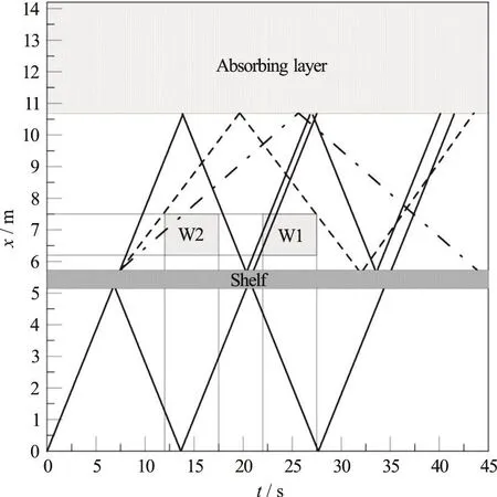
Fig. 2 Paths of free wave fronts in the space-time domain. Solid line=1st harmonic, dashed= 2nd harmonic, dotted-dashed=3rd harmonic. W1: data windowing for the 2nd and 3rd harmonic, W2: data windowing for the 1st harmonic only.

Figure 2 shows clearly that there is no chance to get a space-time window that (1) allows a complete development in space of the full set of harmonics, (2)and that is totally free from multiple reflections for any harmonic component. The latter requirement is hard to achieve especially for the first fastest harmonic. Since the interest of this study is mainly on the higher order terms, the space-time window selected is 6.2 m≤x≤7.5 m and 22s≤t≤27.5s , marked as W1 in Fig. 2.

The Parameter Identification is able to distin- guish between waves of the same frequency traveling in opposite directions but cannot distinguish between waves of the same frequency traveling in the same direction.This is the case of the first harmonic over the window W1 specified above. Indeed the first harmonic shows multiple reflection between the beach and the shelf.For this reason, we have used an additional space-time window for the first harmonic only, i.e., 6.2 m≤x≤7.5 m and 12s≤t≤17.5s , marked as W2 in Fig. 2.

According to the space-time length of W1 and W2 and according to the numerical resolution of the simulations in space and time, in the present application the number of simultaneous stations Nstationsis of order of 102and the number of consecutive time steps Ntimeis of order of 5×102, thus the total number of reference elevations within the space-time window used in Eq. (4) is of order 104.

The simulations have been conducted without shelf too, in order to check the actual amplitude of the incoming wave train. Here the time window is again 12s≤t≤17.5s (W2). Figure 3 shows a snapshot of the free surface at time t=12s with and without the shelf.

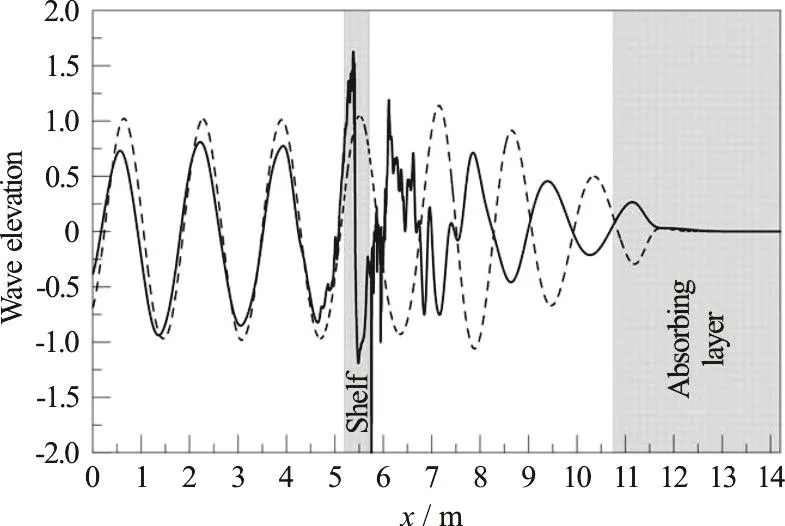
Fig. 3 Elevation of the free surface along the basin, t=12 s,with (solid) and without (dashed) shelf. Case S1, highest incident wave steepness tested; wave breaks at the shelf

Finally, within the selected window, a further data windowing has been applied for the standard Fourier analysis (see below). At each station x, 5 complete (main) wave periods T=1/f have been used, so that the Fourier analysis has been applied formally at its best.

2. The simulation framework

The momentum and mass conservation of an incompressible Newtonian fluid hold. No heat exchanges are here considered. The differential formulation reads as follows

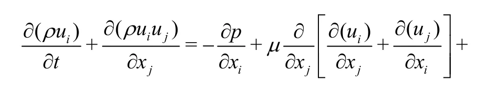
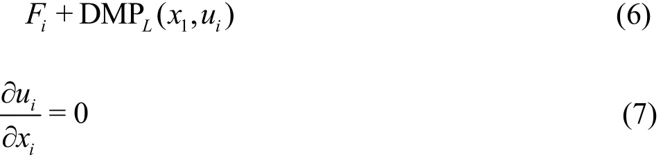
where ρ is the fluid density (Eq. (11)), uiis a velocity component, p is the pressure, μ is the dynamic viscosity (Eq. (10)),iF are the body forces ,(0,-ρg,0), t and xiare time and space independent variables. The last extra term DMPL(x1, ui) in Eq. (6) is introduced in a specified zone of the domain to dampen waves as discussed below.

The problem considered faces a two-phase flow,air and water, where the treatment of the free surface can be ensured with an additional formulation(Scardovelli and Zaleski (1999)). The interface capturing VOF method of Hirt and Nichols (1981) is here adopted (Eq. (8)), with the artificial velocity method proposed by Rusche[19]

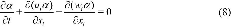
where α is the volume fraction and wiis an artificial velocity field that is directed normal to and towards the interface. The relative magnitude of the artificial velocity is determined with the following expression

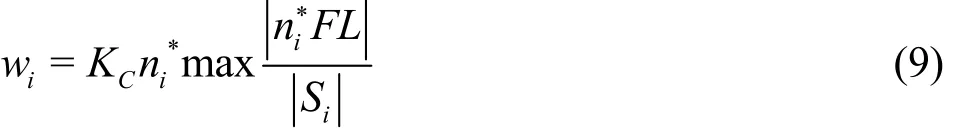
where KCis an adjustable coefficient that determines the magnitude of the compression, ni*is the interface unit normal vector, FL is the flux and Siis the surface area vector. In this work KChas been set to 1 after a series of tests aimed to ensure mass conservation in relatively long time integration.

The following properties hold

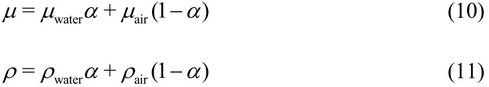
The extra term DMPL(x1, ui) in Eq. (6) is used for wave absorption in the damping zone. In the present study DMPL(x1, ui) is set equal to ραvd(x1) uiwhere vdis an artificial viscosity enabled only on the specified zone represented schematically in Fig. 1.The characteristic feature of this method is that, to some extent, there is no need to specify the spectral content of the incident wave train. The method thus works rather efficiently also for non-monochromatic waves, provided the beach length is set longer than the typical (longest) wavelength in the wave train. See Fig.3 as a sample case. The implemented artificial viscosity term vd(x1) is defined as a function of the longitudinal position x1, increasing from zero to its final value at the outlet, growing smoothly from the beginning of the sponge layer up to the end of the domain. Details of the performances of the wave damper as implemented by the authors can be found in Contento et al.[20].

Equations (6)-(8) represent the complete mathematical formulation of the two phase flow model.They are solved within the OpenFOAM framework[12],with a Finite Volume technique, using the schemes summarized in Table 2, with a 2nd order Gaussian integration. The pressure-velocity coupling is achieved using a pressure implicit with splitting of operator(PISO) algorithm. The Euler implicit scheme is adopted to march forward in time. The free-surface location is computed using the Multidimensional Universal Limited for Explicit Solution (MULES)method. Additional info on the present implementation can be found in Lupieri and Contento[21].

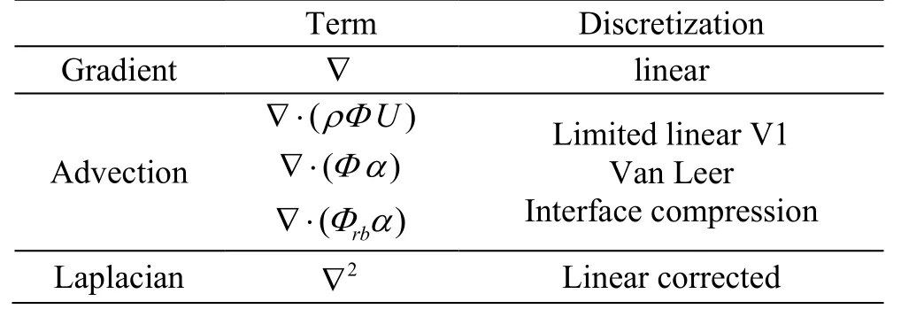
Table 2 Numerical schemes in use in the simulations

The computational domain has been set in order to reproduce the experiments of Grue[2]in 1:1 scale.The space discretization has led to a computing hybrid grid of more than 2×106cells. The air-water interface region has been discretized with approx. 102vertical elements per incident wave height, whereas the horizontal discretization has been set to 2×103elements per undisturbed wave length at the shelf, around 4×102in the far field. At the shelf wall, the first grid cell is positioned at y+=1, with reference to the incident wave flow. The growth rate to the outer layer is imposed with respect to standard ITTC recommendations. A detail of the grid at a corner of the shelf is presented in Fig. 4.

As for the influence of turbulence on wave propagation, transformation and ultimately breaking,the literature and scientific discussion on this topic are notoriously ample. In 3-D cases, even LES model may not be the ultimate solution, as discussed by Christensen[23]. In 2-D cases the adoption of RANS or LES models introduces further theoretical inconsistencies.

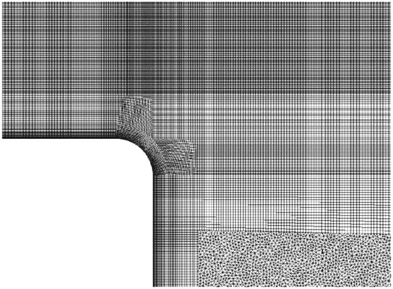
Fig. 4 Zoom of a detail of the computing grid at the shelfʼs corner: please note that the radius at the corner is approximately 82 times smaller of the shelfʼs vertical extension

The present work is focused on the wave transformation of mildly breaking 2-D waves and specifically on the non-linear behavior of the longitudinal properties of higher order harmonic components(phase speed of free waves generated at the shelf). In general, the present case study is characterized by a very low Reynolds number, ≈104or less, and turbulence is expected to play a role possibly in a very small region of the domain around breaking. The results obtained by Grue[2]with an inviscid nonlinear model confirm this. Lupieri and Contento[21-22]have studied three typologies of 2-D steady and unsteady breakers and specifically the interaction of regular waves with a 2-D circular cylinder at low Keulegan-Carpenter numbers, in diffraction regime, with mild breaking. In those studies the grid typology and fineness was very similar to that adopted in the present work and a very small or even null eddy viscosity gave the best results. For these reasons, here we have followed the same approach i.e., the simulations have been conducted without turbulence model,the grid adopted ensuring a reasonable resolution at the air-water and fluid-body interfaces. For sake of completeness, the simulations of case S1 of Table 1 have been conducted with a standard k-ω SST model too. The results obtained show a low quality,they will be commented only and not shown in the plots.

3. Results and discussion

Figures 5, 6 show a temporal sequence (waterfall)of free surface profiles over a representative portion of the domain and for 5 complete stationary wave periods. Cases S1 and S5 of Table 1 have been selected as representative of a breaking (S1) and non-breaking (S5) conditions respectively. The strong wave transformation at the shelf and the complexity of the free surface elevation at the lee side of the shelf are clearly evidenced by the complex pattern of rays.Still, the overall space-time periodicity in the far field of the lee side is kept, even in breaking conditions(S1).

Fig. 5 (Color online) Waterfall of free surface profiles over a portion of the domain, case S1. The free-surface elevation is scaled by a factor 4

As reported by Shen and Chan[24], in a periodic incident flow past an obstacle, the presence of already detached structures relatively close to the boundary layer of the object can alter the symmetry of the separation mechanism, for instance introducing a delay. At the weather corner of the shelf in the cases here analyzed, vorticity aggregations with opposite sign are created and travel towards the free surface or drift in the outer domain, whereas dipoles originated at the lee corner of the shelf have never been observed to interact with the free surface. The vorticity at the free surface comes from the shear located under the bulge of the breaking wave, as described for instance by Iafrati and Campana[25]in the case of submerged foils.

The weather side of the shelf in the selected window W1 for case S1 is here analyzed. Following the notation of Williamson and Roshko (1988) in which ”S” denotes a single vortex detached and ”P” a pair, Table 3 reports the sequence observed, splitting each period (from I to V) in two half cycles (1/2 +1/2). As in the case of a horizontal cylinder in a wavy flow at low Keulegan Carpenter number investigated by Lupieri and Contento[21-22], the local detachment of a sequence of vortices of the same sign (+ or -) may take place, denoted as a ”roll up” in the present table after Otsuka and Ikeda (1996).

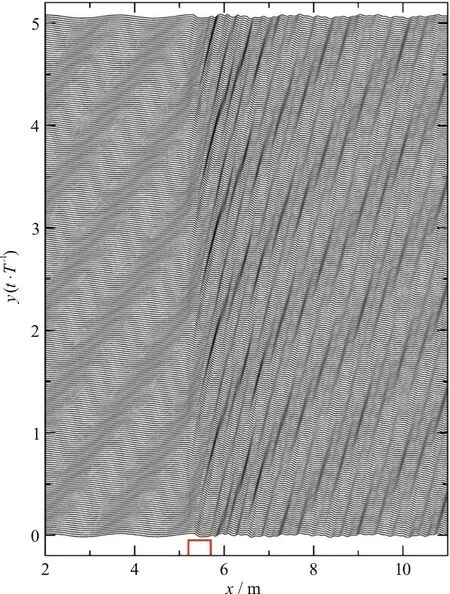
Fig. 6 (Color online) Waterfall of free surface profiles over a portion of the domain, case S5. The free-surface elevation is scaled by a factor 4

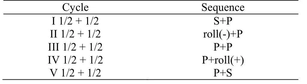
Table 3 Case S1: Sequence of vorticity structures detached from the weather side corner of the shelf

Figure 7 shows a snapshot of the free surface profile and of the non-dimensional vorticity contour for a spilling breaker (case S1, cycle I, first half cycle).In this case, the fluid close to the free surface at the lee side exhibits the chaotic layer of vortex structures induced by breaking and responsible for the small amplitude fluctuations of the free surface. A single vortex (S in Table 3) is shown while detaching at the weather side. Dipoles, already present in its proximity,are advected to interact mildly with the free surface.

At the lee side of the shelf, the large scale clockwise rotating vortex, induced by the mean positive flow above the shelf, spans from the free surface to the bottom of the basin. These phenomena are necessarily all related to the mechanism of wave transformation but still play a minor role with respect to the birth and death of higher order waves, the former being basically of inviscid nature Grue[2], the latter being of viscous origins with increasing impact with increasing incident wave amplitude.

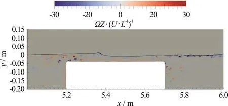
Fig. 7 (Color online) Incipient spilling breaking and non-dimensional vorticity contour, case S1

3.1 Amplitude spectrum of the wave elevation along the basin

A standard Fourier analysis is applied to the wave elevation η(t) at the lee side, for any x independently. Following the data windowing described in Section “Data windowing”, it provides the distribution of local amplitudes. Figures 8(a), 8(c) show a selection of results, cases S1, S3 and S6 respectively. In the same plots, the experimental data from Grue[2]are reported as symbols and thin horizontal lines. These data have been provided by Grue as space averages at the lee side thus the position x of the symbols is meant as reference only. Here they are ideally positioned in the middle station of W1/W2.

As for the first harmonic a1, it has been derived on the space-time window W2 for all cases but S4 and S6. For S4 and S6 it has been derived on W1 (see Fig.2) on purpose. W1 and W2 share the same space window but they refer to two different time windows.As expected, on W1 (Fig. 8(c)) the first harmonic shows clearly the effect of the choice of the wrong data window. Indeed the method adopted for now does not distinguish between free f, locked l or reflected R waves with the same frequency, thus the local amplitudes are simple super-positions of f, l or R components. On the contrary, Figs. 8(a), 8(b)show a clean condition for the analysis, i.e., the adoption of W2 guarantees a data analysis free from reflections for the first harmonic.

As for the second harmonic a2, it has a rather flat shape over the entire basin (case S3 apart), and mostly over W1. The third harmonics a3is clearly still under development along the basin, however its steadiness over W1 is acceptable. As for the fourth harmonics a4, cases S2, S3 and S4 show a clear decay of the amplitude with the direction of wave propagation. Looking to higher orders, the Fourier transform shows that for the steepest incident waves there are non-negligible amplitudes on the lee side up the 7th harmonic (not shown here).

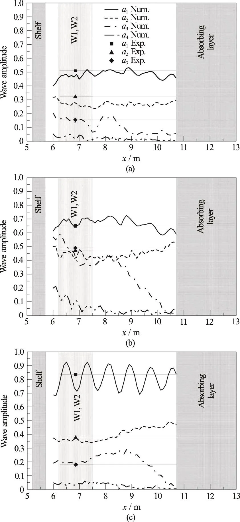
Fig. 8 Standard Fourier analysis of the wave elevation along the basin, case S1(a) and S3(b) on W1/W2, S6(c) on W1 (see Fig. 2), lines = numerical results, symbols = exp. data from Grue[2]. The experimental data are space averages at the lee side. Here they are ideally positioned in the middle station of W1/W2 and then represented with a thin horizontal line

As discussed above, this local harmonic analysis is not able to distinguish between free, locked and reflected waves. Thus the results obtained with this analysis of the wave elevation at independent stations must be interpreted on an space-average basis. Within these hypotheses, the results obtained compare reasonably well with the experimental data, but still they lack more detailed information on the wave energy transfer to free or bound components.

3.2 Reduced model and parameter identification

3.2.1 Amplitudes of free, locked and reflected waves A deeper analysis of the wave characteristics at the lee side of the shelf has been conducted according to the methodology described in Section “Model reduction” and “Parameter identification”. Provided the reduced model ηMODEL(xi, ti)is representative of the physical phenomenon, the PI applied to the entire matrix ηSIMUL(xi, ti)at i=1,Nstationsand at j=1,Ntime, allows to distinguish between free, locked and reflected waves intrinsically, at any order.

A preliminary Parameter Identification has been applied assuming that the component waves, whichever they are among free, locked and reflected, behave linearly in the dispersion relation. Thus, in this preliminary run the Parameter Identification has been applied to amplitudes and phases only. As explained above, the analysis has been conducted on the time space-time windows W1 (for higher order waves) and W2 (for first order wave) of Fig. 2.

A reasonably good fitting has been successfully achieved for the cases S5 to S7 only, i.e., for the smallest amplitudes of the incident wave a. The comparison with the results of Grue[2]confirms the quality of the results obtained for these three cases.However any further attempt to make the reduced model ηMODEL(xi, ti)represent the physical phenomenon also for the cases with higher incident wave amplitude a has failed.

From a bare visual observation of the reconstructed wave profiles in the space-time domain and from the comparison with the original data from the simulations, it has come to evidence that higher order free waves travel much faster than expected from the linear dispersion, though being still of very small steepness (≈10-2). Thus the number of parameters of the reduced model ηMODEL(xi, ti)has been changed so that the wave numbers of free and reflected waves take part to the fitting procedure as free parameters.

The results obtained are shown in Fig. 9. With this set-up of the reduced model and its parameters,component wave amplitudes now compare extremely well with the experimental results of Grue[2]for anyorand at any order. The PI has proved very robust and with great reliability on the set of parameters obtained.

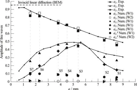
Fig. 9 Non-dimensional free wave amplitudes (solid and empty large symbols) Vs incident wave amplitude a, obtained from the Parameter Identification method. Exp. data from Grue[2] are shown with solid lines and small symbols. The result form inviscid linear diffraction obtained by a time domain BEM code is shown too (horizontal dashed line). The non-dimensionalization is made according to the values of the incident wave amplitude without shelf

As observed experimentally by Grue[2], the non-dimensional amplitude of the first harmonic af,1reduces its magnitude progressively with the increasing incident wave amplitude a. The reflected first order waveis almost negligible on window W2.

As for the higher order harmonics, the second af,2and third af,3order free waves specifically,they increase their non-dimensional magnitude until the limit of incipient breaking of the whole wave,around S3 (spilling mode). In this strongly nonlinear condition, the second and third order free waves reach almost the same amplitude. For any further increase of the incident wave amplitude a, their non-dimensional magnitude decreases progressively.

For sake of completeness, the fourth order free wave af,4is shown too. It exhibits non negligible amplitudes (10 percent of the incident wave) mostly for the cases S3, S4 and S5. Locked waves amplitudes al,iand phases have been captured by the reduced model. Their amplitudes is always extremely small,approximately two orders of magnitude lower than af,1. They are not shown here.

As for the results with turbulence model k-ω SST for case S1, the data obtained from the PI are the following: a=0.508268, aR=0.047555, a=f ,1f ,1f,20.400608, af,3=0.006794and finally af,4=0.004794. They are not shown in Fig. 9 for sake of clarity. af,1overestimates slightly the experimental value,af,2is well over and af,3,af,4are really small. The turbulence model acts as a low pass filter at breaking, enhancing the first and second harmonics and killing the rest of the harmonic content.

3.2.2 Phase speed of free waves

Further strong nonlinear effects induced by the interaction of the wave train with the shelf are found in the phase speeds, or in the related wavenumbers, of the component free waves. The PI, applied to the reduced model proposed, has given the results presented in Fig. 10. The plot shows the non-dimensional phase speed of each free wave component against the incoming wave amplitude a. The non-dimensionalization of phase speed is obtained with reference to the corresponding values from linear theory.

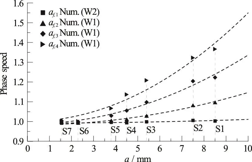
Fig. 10 Non-dimensional phase speed of free waves Vs incident waveamplitude a.Thenon-dimensionalizationis made according to the values from linear theory

The phase speed increases almost quadratically with a for any component, with increasing difference from linearity with the increasing frequency of the wave component. This might be thought as a standard (Stokes) nonlinear effect induced by the increasing steepness of each component. However,looking at the wave steepness as derived from the Parameter Identification (Fig. 11), it is limited by very small values and its behavior is clearly not monotonic with a, with a break point at S3 approximately. Indeed,wave breaking that starts in spilling mode around S3 reduces progressively the steepness of any component wave, at any order. Thus the effect of wave steepness is not so directly related to the increasing phase speed observed in these results.

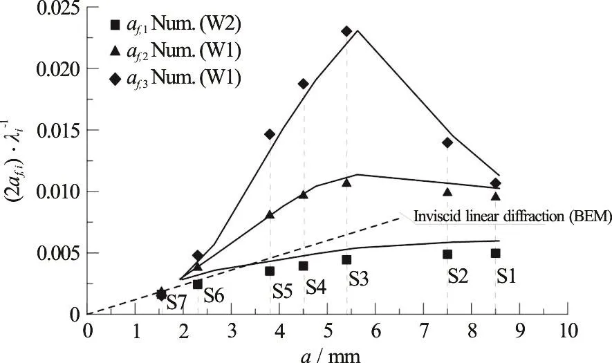
Fig. 11 Wave steepness of free waves Vs incident wave amplitude a (solid lines with symbols). The result form inviscid linear diffraction obtained by a time domain BEM code is shown too (dashed line)

This increased phase speed recalls the coalescence of higher order waves observed in focusing waves. Chaplin (1996) and Contento et al.[21]have studied experimentally and numerically respectively the phenomenon obtained by frequency focusing of a given spectrum. Their results show that in quasibreaking conditions, around the focusing region, the higher order waves generated outside the input band have an almost constant phase speed equal to the value of the upper frequency in the input band, i.e.,the imposed coalescence of in-phase wave components makes the main features of the overall wave dominant in almost the whole spectrum.

4. Conclusions

In this work, the wave transformation of regular small-amplitude quasi-monochromatic waves induced by the interaction with a shallowly submerged rectangular shelf has been studied by means of numerical simulations based on the two-phase flow Navier-Stokes equations, solved with the Finite Volume method and the Volume of Fluid interface capturing method.

The set-up of the simulations has been built in order to reproduce to full-scale the experiments from Grue[2].

The analysis of the results has been carried out initially by a standard Fourier transform at any virtual probe on the free surface. A more detailed analysis has been achieved applying a Parameter Identification technique (PI) to a reduced model, using an extremely large space-time matrix of wave elevations.

The combination of reflection, transmission,breaking, seiching makes the global behavior of the free surface highly unsteady in a basin of reduced longitudinal size. Still, the PI has performed successfully in capturing a complex superposition of free,locked and reflected waves, allowing a robust decomposition of the phenomenon.

The results have shown a variety of nonlinear effects, spanning from those related to inviscid flow features up to wave breaking. The energy transfer to higher order terms has been clearly identified and successfully compared with experimental data. In particular the PI method applied on a well-based data window has made the consistent detection of amplitudes of free, locked and reflected waves possible, at any order. The method has also evidenced the strong nonlinear effects on the phase speed of free higher order waves, a kind of coalescence of component waves induced by the shallow water region above the shelf.

Acknowledgements

The “Programma Attuativo Regionale del Fondo per lo Sviluppo e la Coesione (PAR FSC 2007-2013)Linea 3.1.2” is acknowledged for providing the support of the OpenViewSHIP Project.