Weibin DAI,Jun ZHANG,Xiaoqian SUN

aSchool of Electronic and Information Engineering,Beihang University,Beijing 100083,China

bNational Key Laboratory of CNS/ATM,Beijing 100083,China

cBeijing Key Laboratory for Network-based Cooperative ATM,Beijing 100083,China

On solving multi-commodity flow problems:An experimental evaluation

Weibin DAI,Jun ZHANG,Xiaoqian SUN*

aSchool of Electronic and Information Engineering,Beihang University,Beijing 100083,China

bNational Key Laboratory of CNS/ATM,Beijing 100083,China

cBeijing Key Laboratory for Network-based Cooperative ATM,Beijing 100083,China

Multi-commodity flow problems(MCFs)can be found in many areas,such as transportation,communication,and logistics.Therefore,such problems have been studied by a multitude of researchers,and a variety of methods have been proposed for solving it.However,most researchers only discuss the properties of different models and algorithms without taking into account the impacts of actual implementation.In fact,the true performance of a method may differ greatly across various implementations.In this paper,several popular optimization solvers for implementations of column generation and Lagrangian relaxation are discussed.In order to test scalability and optimality,three groups of networks with different structures are used as case studies.Results show that column generation outperforms Lagrangian relaxation in most instances,but the latter is better suited to networks with a large number of commodities.

©2017 Chinese Society of Aeronautics and Astronautics.Production and hosting by Elsevier Ltd.This is an open access article under the CCBY-NC-NDlicense(http://creativecommons.org/licenses/by-nc-nd/4.0/).

1.Introduction

The multi-commodity flow problem(MCFP)deals with the assignment of commodity flows from source to destination in a network.MCFPs are highly relevant in several fields including transportation1and telecommunications.2

MCFPs have been studied by a number of researchers for several decades,and a variety of solutions have been proposed such as column generation,Lagrangian relaxation,branchand-bound,and Dantzig-Wolfe decomposition.Tomlin3presented a column generation algorithm first,and he is also one offorerunners of using Dantzig-Wolfe decomposition.Based on these methods,a number of new processes were proposed more recently.For instance,Barnhart et al.presented a partitioning solution approach in order to solve large-scale MCFPs with large numbers of commodities.4Many constraints can be relaxed with a cycle-based formulation and column generation.Then,by solving a series of linear programs with reduced size,an optimal solution can be obtained within a finite number of steps.Based on column generation,Barnhart et al.presented a modified version of the branch-andbound algorithm for solving origin-destination integer multi-commodity flow problems.5An algorithm for path-based models was improved by presenting a new branching rule and adding cuts.Computationalcomplexity can be reduced significantly by these cuts in many real-world situations.The classical column generation algorithm has a variety of advantages for solving MCFPs.However,because the restricted master problem(RMP)changes a lot with continuous column generation iterations,the solution often convergences slowly.Therefore,Gondzio et al.proposed the primal-dual column generation method(PDCGM)for solving this problem.6–8PDCGM is a modified method relying on the sub-optimal dual solutions of restricted master problems where solutions are obtained with the primal-dual interior-point method.This method was initially developed for solving large-scale convex optimization problems.PDCGM was shown by the authors to be competitive and suitable for a wide context of optimization problems.

In addition to column generation,new methods based on Dantzig-Wolfe decomposition and Lagrangian relaxation have been developed.Based on Dantzig-Wolfe decomposition,Karakostas proposed polynomial approximation approaches in order to solve MCFPs.9These approaches were also derived from other previous algorithms.10,11These methods minimize computation time dependence on the number of commodities.Based on Lagrangian relaxation,Retvari et al.proposed a new Lagrangian relaxation method that can solve the MCFP as a sequence of single-commodity flow problems.12This technique performs best when solving OSPF(open shortest path first)traffic engineering problems because a given path can be improved towards approximate optimality while giving several necessary parameters.In addition,Babonneau and Vial proposed a new method based on partial Lagrangian relaxation,13which constrains relaxation to the set of arcs that are saturated at the optimum.This method can be used to solve large problems.

In addition to the previous research,modified versions of MCFPs are also studied.Moradi et al.proposed a new column generation method for solving bi-objective MCFP problems.14Based on the simplex method and Dantzig-Wolfe decomposition,the algorithm moves between different points.Similar to Karakostas’s method,it demonstrates that the average computation time does not necessarily depend on the number of commodities.Path-based models are often used to solve MCFPs;However,Bauguion et al.proposed a new idea about such models.15,16Instead of generating paths for each commodity,they generated groups of paths in other ways,such as combining them into single sets or separate trees.These methods reduce computation time compared with other models.

MCFPs can be applied to many different application problems.17Zhang et al.presented a multi-commodity model for supply chain networks,18which was solved using the Benders decomposition method.Caimi et al.studied the problems of conflict-free train routing and scheduling and proposed a new resource-constrained modelbased on the multicommodity flow.19Morabito et al.studied network routing for generalized queuing networks and presented a multicommodity flow algorithm based on a routing step and an approximate decomposition step.20Shitrit et al.applied the multi-commodity flow problem to tracking of multiple people.Experimental results showed that their approach performs better than other state-of-the-art tracking algorithms.21

As our review of related literature shows,the vast majority of the methods proposed for solving MCFPs discussed the properties of different models and algorithms without considering the impact of implementation.For instance,while solving the MCFP with an algorithm,some portions of the problem can be formulated as a linear program.In this case,it is important to select the appropriate implementation type,i.e.linear program solver.22This paper introduces the formulations and processes of two commonly-used algorithms for solving MCFPs:column generation and Lagrangian relaxation.In addition to the algorithm theory,implementations for MCFPs are also discussed.Several popular program solvers,such as GNU linear programming kit(GLPK),CVXPY,GUROBI,and SCIPY,are introduced briefly.Past research often performed comparisons with single,outdated competing methods or implementations.This paper promotes the idea of comparing popular methods in order to decide which one is the best for a given problem.In order to test the scalability and optimality of the algorithms and program solvers,three groups of networks(grid,planar,and airport networks)are chosen as case studies.For each group of networks,the optimality,computation time,and number of iterations for the algorithms and different program solvers are compared.

Results indicate that column generation has better properties for solving an MCFP than Lagrangian relaxation in most instances.However,Lagrangian relaxation can be faster and within acceptable optimality bounds in certain large-scale networks with a high number of commodities.There is a similar relationship with implementations for column generation:CVXPY performs better than GLPK for solving MCFPs with a large number of commodities by column generation while GLPK is superior for a small-scale MCFP.This work shows the tremendous impact ofimplementation techniques on computation time and solution quality and lays the foundation for further research on MCFPs.

The remainder of this paper is organized as follows:An introduction and formulation of the multi-commodity flow problem are provided in Section 2.Relevant solution techniques,such as column generation,Lagrangian relaxation,and several program solvers,are introduced in Section 3.In order to compare these techniques,three groups of different datasets are discussed in Section 4.The evaluations performed using these datasets as case studies are presented in Section 5.Conclusions are in Section 6.

2.Multi-commodity flow problem

The MCFP seems like a combination of several singlecommodity flow problems.However,because of the interaction between commodities,the complexity of MCFP is much higher than that for solving each single-commodity flow problem independently.23In order to solve MCFPs,two necessary constraints must be considered.The first is the travel demand,which means that all the commodities need to be transported to their destinations.The second is the edge capacity constraint.This means that the flow on each edge can not exceed flow capacity.The first constraint is essentially the sum of a set of single-commodity flow problems.However,the second constraint needs to consider all commodities together,and it causes interactions between them.G=(V,E)is a directed network.HereVandEare the set of nodes and edges with sizesnandm,respectively.For each edgel,there is a costcland capacity capl.tkinds of commodities need to be transported from their origin nodes to destination nodes.O(k)andD(k)are used to represent origin and destination node of commodityk.24In addition,dkis the travel demand of commodityk.An optimal flow assignment with minimum cost must be found to satisfy the travel demand and capacity constraints for this problem.Thus,the MCFP can be formulated as follows25:

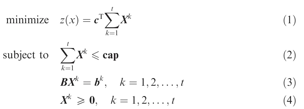
where Eq.(1)is the objective function of total cost.Eqs.(2)and(3)are an edge capacity constraint and node flow equilibrium equation,respectively.Eq.(4)isa non-negative constraint.

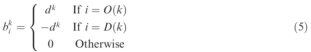
Here,Xk=[x1,x2,...,xm]Twithk=1,2,...,tis the flow vector of each edge for commodityk.The vectors of cost and capacity on each edge are represented by c=[c1,c2,...,cm]Tand cap=[cap1,cap2,...,capm]T,respectively.26The incidence matrix between nodes and edges is indicated by B=[Bil]n×m.It has a size ofn×mand can be defined by listing all edges then,for thelth edge(i,j),settingBil=1 andBjl=-1;bk=defined as follows:27

A small example,shown in Fig.1(adapted from Ref.2),and Table 1 are discussed as a case study.There are 6 nodes,10 edges and 3 commodities in this network.The number pair on each edge represents the pair of cost and capacity.

For each commodityk,the travel demand must be satisfied.This means that we need to find a set of paths betweenO(k)andD(k),and their total flows are equal to the travel demand.In addition,due to edge capacity constraints,the complexity of MCFP is much higher than the combination oftsinglecommodity flow problems.

The optimal solution of this small problem is shown in Table 2,and the optimal value of the objective function is 43.The results in Table 2 can also be represented with the path flows shown in Table 3.

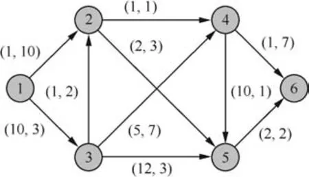
Fig.1 A small example.

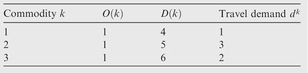
Table 1 Sample commodities.

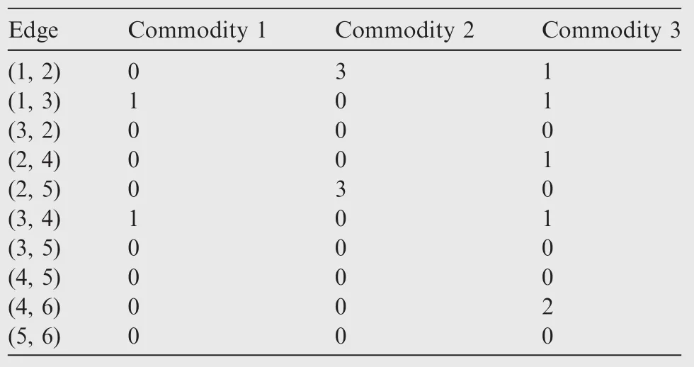
Table 2 Solution I for the small example.

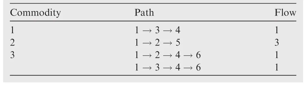
Table 3 Solution II for the small example.

Note that only a few edges and paths contribute to the optimal solution for each commodity.Flows on a majority of edges and paths are zero.For instance,edge(3,5)is not used at all.This property shows the potential for solving MCFPs more efficiently.

3.Solution techniques

Section 2 shows that the formulation of the MCFP has a structure that should be exploited during computation of a solution.Eq.(3)can be divided intotindependent equations for each commodityk,directly.Eq.(2)is the only interaction between all the commodities.If the commodities do not influence each other in this constraint,the MCFP can easily be solved through the solution of several independent singlecommodity flow problems.From this concepti,Lagrangian relaxation is proposed for Eq.(2).Just as with the small example in Section 2,most variables do not contribute to the solution.Based on this observation,a column generation algorithm,that only considers a small set of variables is presented.In this section,several techniques including the column generation in Section 3.1,Lagrangian relaxation in Section 3.2,and optimization solvers in Section 3.3 for implementation are introduced.

3.1.Column generation

In Eqs.(1)-(4),there aret×mvariables in the model.However,while solving the multi-commodity flow problem,most variables do not contribute to the optimal solution(see the example in Section 2).In this case,column generation is used to solve MCFP.New columns are added into the solution step by step as necessary to improve the objective function.The process of this algorithm is as follows:

First,a set of initial columns are used to construct the dual problem.The solutions of the dual problem are used to generate price problems for all the commodities.We assume thatis the optimal objective function value of thekth price problem.If≥ 0 for∀k=1,2,...,t,the original MCFP reaches the optimal solution.3Otherwise, if＜0 fork=k1,k2,...,kp,then the solutions of these price problems need to be added as a new column into the set.The algorithm continues running with the steps above until optimal solutions are obtained.

3.1.1.Dantzig-Wolfe decomposition and master problem

A problems is first dealt with using Dantzig-Wolfe decomposition and split into a master problem(containing a set of currently active columns)and a set of sub-problems.

For each commodityk,variable vector Xkcan be decomposed as Xk=coefficients satisfyingΣthat satisfy the following constraints:

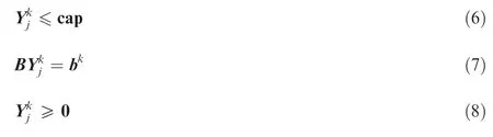
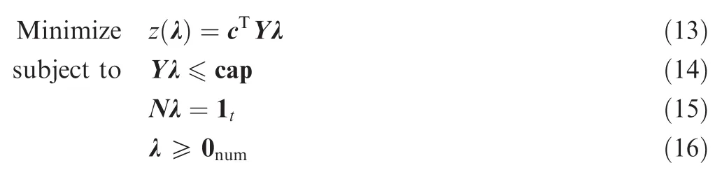
Therefore,the master problem can be formulated as

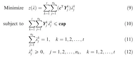
The optimal solution based on this set of columns can be obtained by solving the master problem.However,at this stage it can not be ensured that this solution is also optimal for the original MCFP.Therefore,the dual problem and price problems are solved in the next section.

3.1.2.Dual problem

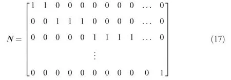
In orderto show the modelclearly,the formulation Eqs.(9)-(12)are transformed into matrix form.

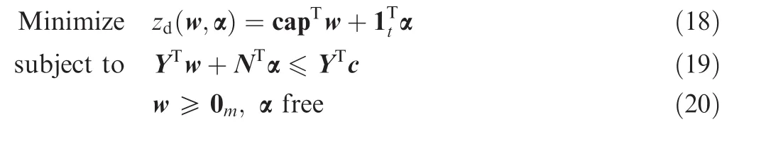
The vectors of dual variables for Eqs.(14)and(15)are indicated by w=[w1,w2,...,wm]Tand α =[α1,α2,...,αt]T,respectively.Therefore,the dual problem of Eqs.(13)-(16)can be formulated as

3.1.3.Price problems

The optimal value of dual variables w and α can be obtained by solving the dual problem from Eqs.(18)-(20).In order to make sure of the optimality of the master problem’s solution and adding of new columns,the price problems need to be solved.For each commodityk,the price problem is formulated as

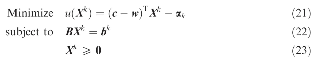
We assume thatis the optimal value ofu(Xk)with constraints Eqs.(22)and(23).Then,it is proven2that the original MCFP can obtain the optimal solution if≥0for∀k=1,2,...,t.

If＜0 fork=k1,k2,...,kp, thenwithk=k1,k2,...,kpneeds to be added into the column set as new columns.A new dual problem and price problems will then be constructed.A loop will continue with these steps until the optimal solution is obtained.

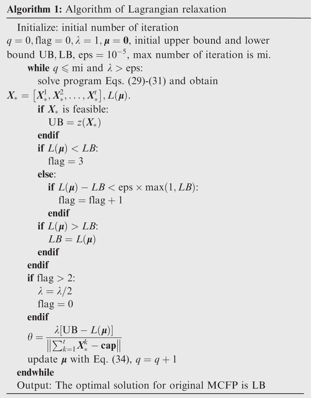
3.2.Lagrangian relaxation

In addition to column generation,Lagrangian relaxation can also be used to solve the MCFP.Lagrange multipliers move towards the optimal value step by step for objective functions closer to optimal.The process is shown as follows:

First,we solve the initial Lagrangian sub-problem with initial Lagrange multipliers.Then,in each iteration,the solution of the sub-problem is used to update the multipliers,and a new solution is obtained by solving the sub-problem with new multipliers.The objective function value will be close enough to the optimal solution if the number of iterations is large enough.The details of this algorithm will be introduced in the following section.

3.2.1.Lagrangian sub-problem

Let μ =[μ1,μ2,...,μm]Tdenote Lagrange multipliers of Eq.(2),then the Lagrangian sub-problem can be generated as follows:

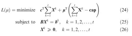
Equivalently,Eq.(24)can also be formulated as

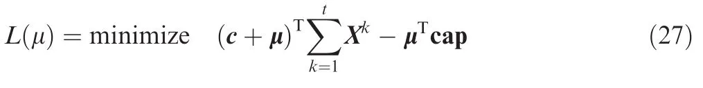
Ignoring the fixed term-μTcap,Eq.(27)is reformulated as

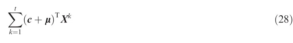
Therefore,the linear program of Eqs.(25),(26)and(27)can be split intotindependent sub-problems for each commodity(k=1,2,...,t)as follows:

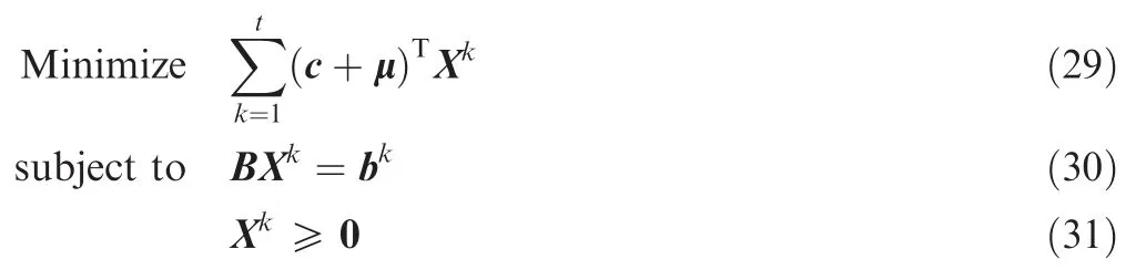
By solving these,the optimal solution for Lagrange multipliers w is obtained.However,this solution may not be optimal for the original MCFP.Therefore,the Lagrangian multiplier problem should be solved.

3.2.2.Lagrangian multiplier problem

It has been proven that the value of Lagrangian functionL(w)is a lower bound on the optimal objective function value of the original MCFP.2Thus,the optimal valuez*for Eqs.(1)-(4)can be formulated as subject to Eqs.(24–26)

In order to solve this problem,researchers often use gradientmethods to approach the optimalsolution.Let X*=be the solution for Eqs.(24)-(26).The multipliers w should be updated as

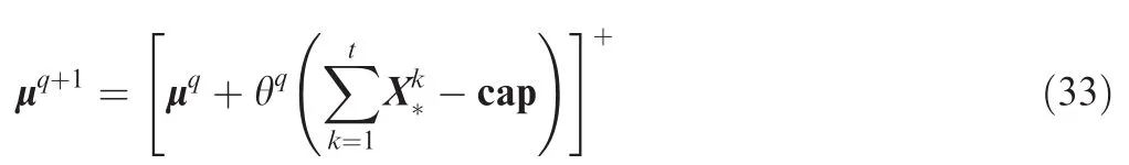
whereqis the number of iterations,θqis a step size and[a]+=max(a,0).

In the next section,the selection of step size is introduced.

3.2.3.Choosing step size

Suitable step sizes are important for solving the Lagrangian multiplier problem.If they are too small,the algorithm may not converge;if they are too large,the optimal solution may be overshot.Therefore,the following conditions should be satisfied:2

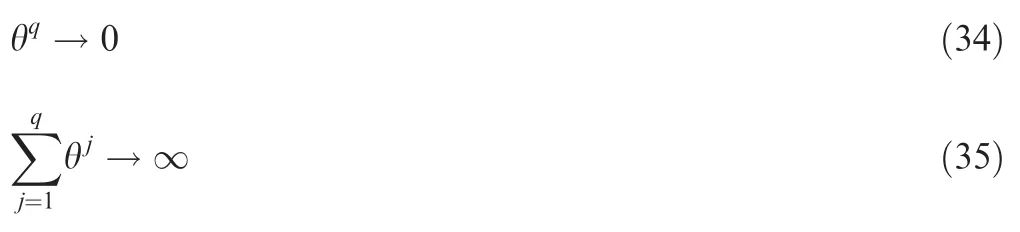
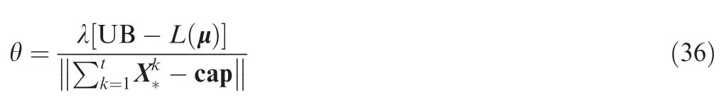
The algorithm of Lagrangian relaxation is shown in Algorithm 1.Its properties will be tested in Section 5.

3.3.Implementations

While implementing the column generation algorithm,the master problem in tion 3.1.1,dual problem in Section 3.1.2 and price problems in Section 3.1.3 are all linear programs.They can all be transformed into the following formulation:

where Eq.(39)is the equality constraint,Aeq and beq are a matrix and a vector,respectively.

The Lagrangian sub-problem in Section 3.2.1 for Lagrangian relaxation is also the same.In order to solve this,it is necessary to find an approximate linear program solver.

Recently,a number of optimizers have become more and more popular,such as GLPK,CVXPY,and GUROBI.There is also one linear program solver,SCIPY.optimize.linprog,in Python.They will be introduced briefly in this section.

3.3.1.GLPK

The GLPK is a package for solving large-scale linear(LP),mixed integer(MIP),and related optimization problems.28

3.3.2.CVXPY

CVXPY is a modeling language embedded in Python for solving convex optimization problems.With this language,the problem can be expressed in a natural way similar to math formulations instead of the standard forms for solvers.29

3.3.3.GUROBI

GUROBI is a commercial optimization solver for linear,quadratic,mixed integer,and several other related programs.Similar to GLPK and CVXPY,it can support a series of program and modeling languages including C++,Java,and Python.30

3.3.4.SCIPY

SCIPY.optimize.linprog is a built-in linear program solver in Python.By inputting the values of objective vectors and constraint matrices in the standard form,linear programs can be solved with this tool.31

Note that Lagrangian sub-problem from Eqs.(29)-(31)for each commoditykis in fact a shortest-path problem.The only difference is that the cost vector c is add by Lagrangian multiplier μ.Thus,the Dijkstra method for finding the shortest path fromO(k)toD(k)can be used in addition to the presented program solvers.The speeds of the Dijkstra method and program solvers all depend on the network size,so their properties will be compared with different kinds of networks in tion 5.

4.Datasets

In order to test the scalability and quality of algorithms and program solvers,three groups of networks,grid networks,planar networks,and airport networks,are chosen as case studies.

The structure of these networks are shown in Tables 4–6.The parameters in the first line are explained as follows:n,m,tare the numbers of nodes,edges,and commodities;pis the edge percentage of all possible edges,i.e.

ADG,ASPLC,ASPLA are average degree,average shortest path length of all the commodities,and average shortest path length of all the node pairs,respectively.

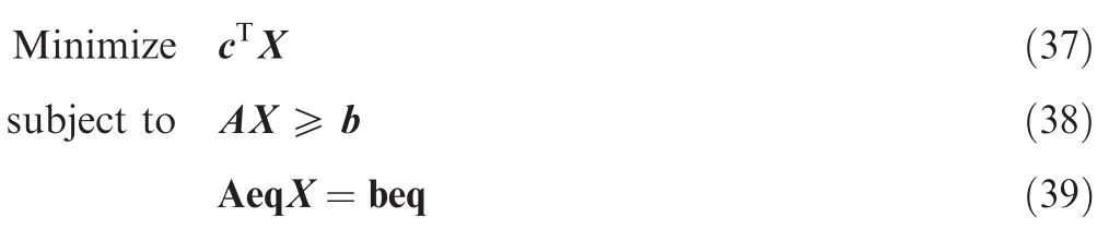
4.1.Grid networks

Nine grid networks are shown in Table 4 withnranging from 25 to 625.With increase of network size,the average degrees all remain small values.Thus,the ASPLC and ASPLA both become larger and larger.this means that for a larger grid network,longer paths are needed to connect two arbitrary nodes on average.

4.2.Planar networks

The properties offive planar networks are shown in Table 5.Average degree values always remain large compared with grid networks.Thus,short paths can be used to connect two nodes.In addition,the commodity numberstof planar networks are much larger than those in grid networks.This means that morecommodities with different OD(origin-destination)pairs need to be transported.

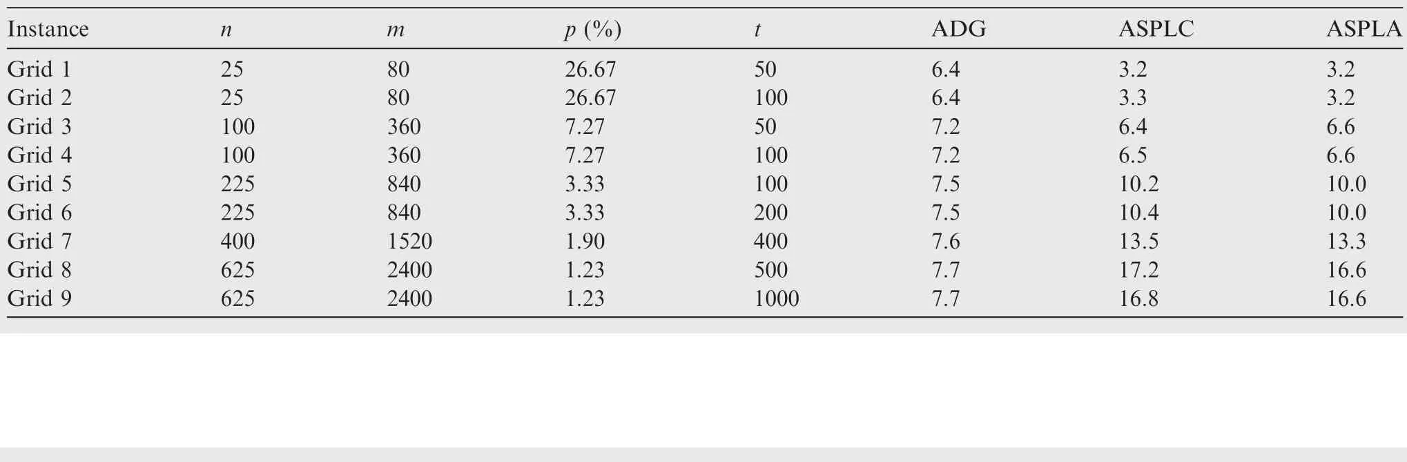
Table 4 Grid networks.

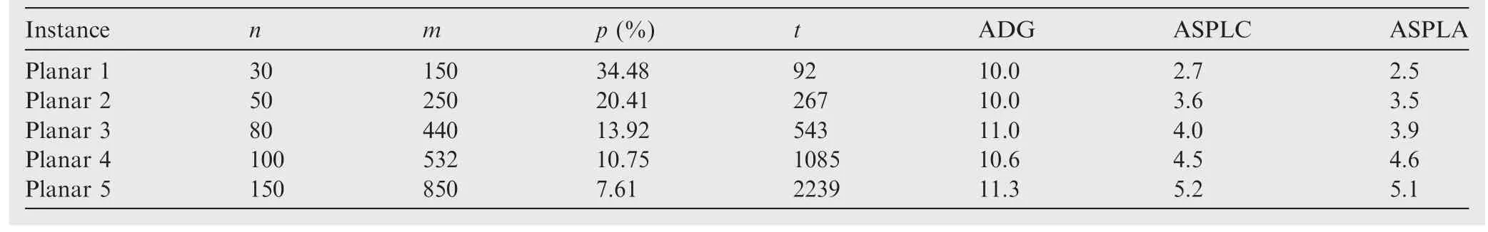
Table 5 Planar networks.

Table 6 Airport networks.

4.3.Airport networks

In addition to the two groups of networks above,several airport networks from different countries are also discussed.As shown in Table 6,the degree average is high,and most OD pairs can be connected in paths with two edges(ASPL＜2).This means that nodes in these networks are strongly connected,which is quite different from grid and planar networks.

5.Evaluation

In this section,the properties of column generation and Lagrangian relaxation with different program solvers are tested on several kinds of networks.In order to compare the quality of each algorithm,a parameter gap is defined as follows:

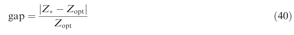
whereZ*is the objective function value of the solution with each algorithm,andZoptis the optimal value of the objective function.In addition to the quality,the computation time and number of iterations are also discussed in this section.

5.1.Grid networks

The gaps of grid networks are shown in Tables 7 and 8.Overall,the quality of column generation is better than that of Lagrangian relaxation.As shown in Table 7,the solutions obtained by column generation are all optimal except for Grid 5 with SCIPY.However,in Table 8,the solutions obtained by the five implementations for Lagrangian relaxation are within 1%of optimality incases where that they can obtain solutions.The computation times for column generation and Lagrangian relaxation are shown in Fig.2.The speed of column generation is faster than that of Lagrangian relaxation with eachimplementation.For column generation,the run time ranking of four implementations is GLPK＜GUROBI＜CVXPY≪SCIPY. For Lagrangian relaxation, it is Dijkstra＜GLPK＜CVXPY＜GUROBI≪SCIPY.In both algorithms,SCIPY has the worst results,and column generation with GLPK is the best choice for solving grid problems.

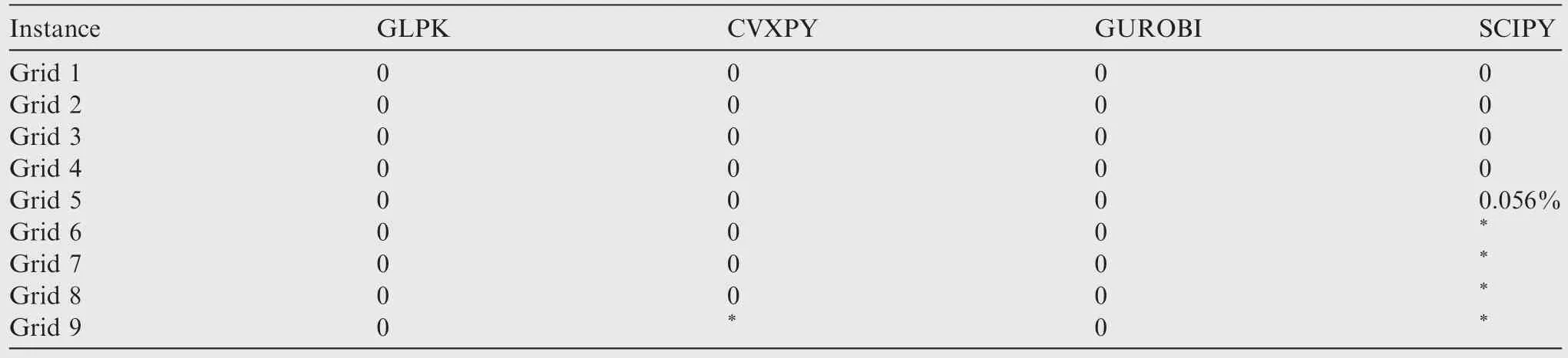
Table 7 Gaps of grid problems with column generation.

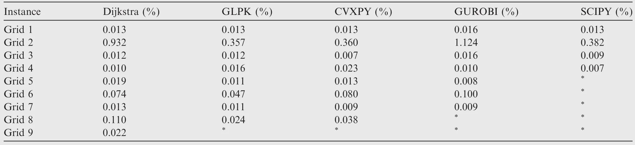
Table 8 Gaps of grid problems with Lagrangian relaxation.

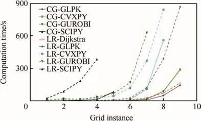
Fig.2 Comparison of computation time for grid networks.

The number of iterations are reported in Tables 9 and 10.It is shown that,for each network,the iteration numbers of column generation are much less than those of Lagrangian relaxation.This may be the major reason for the difference between their computation times.

5.2.Planar networks

In Tables 11 and 12,the gaps of planar networks are shown.Similar to the results for grid networks,solutions obtained by column generation are all optimal except from Planar 3 with SCIPY.Note that the gap of Planar 3 with SCIPY in Table 11 is 51%,and the solution in this case is wrong.This shows that SCIPY is not reliable while solving large-scale linear programs because of its simplicity.The gaps with Lagrangian relaxation in Table 12 are all within 1%of optimality,but are worse than column generation.

The computation time for planar networks is reported in Fig.3.The run time of column generation is shorter than thatof Lagrangian relaxation.Note that the speed of CVXPY is much faster than GLPK with column generation for Planar5 while their run times are similar for Planar1-4.It is shown that column generation with CVXPY is the best for solving largescale networks with similar structure to planar networks.

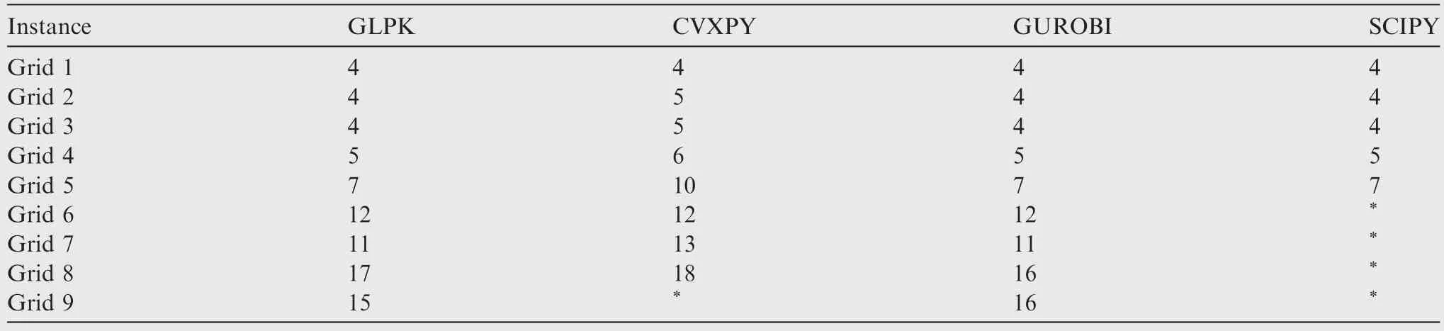
Table 9 Number of grid problem iterations with column generation.

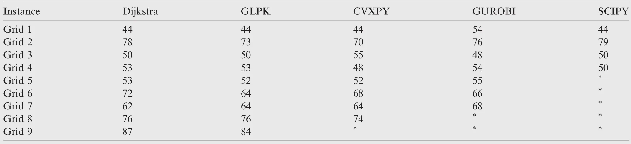
Table 10 Number of grid problem iterations with Lagrangian relaxation.

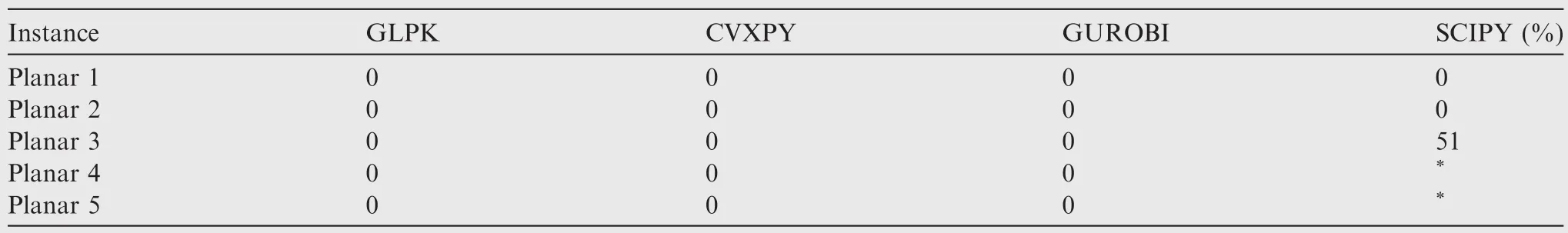
Table 11 Gaps of planar problems with column generation.

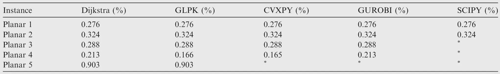
Table 12 Gaps of planar problems with Lagrangian relaxation.

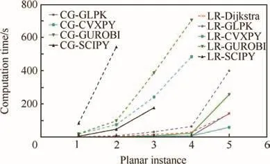
Fig.3 Comparison of computation time for planar networks.

The number of iterations are shown in Tables 13 and 14.Column generation needs many less iterations than Lagrangian relaxation,which is similar to the results of grid networks.

5.3.Airport networks

As shown in Tables 15 and 16,the gaps of airport networks with column generation are generally smaller than those withLagrangian relaxation.The quality of column generation is still better than Lagrangian relaxation.

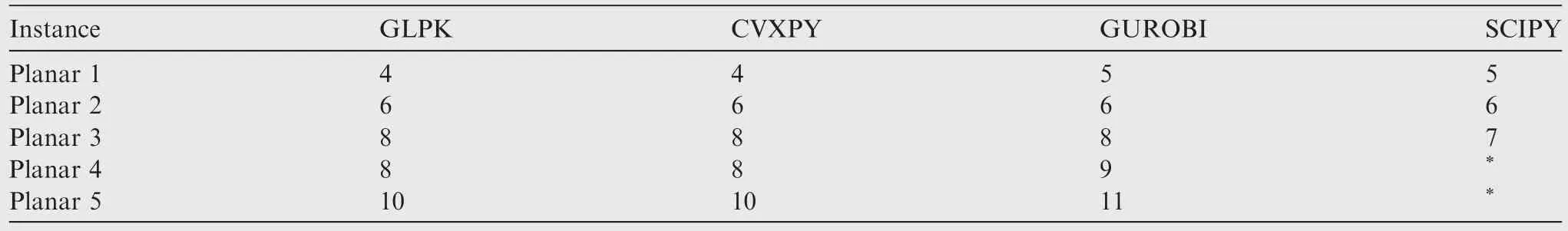
Table 13 Number of planar problem iterations with column generation.

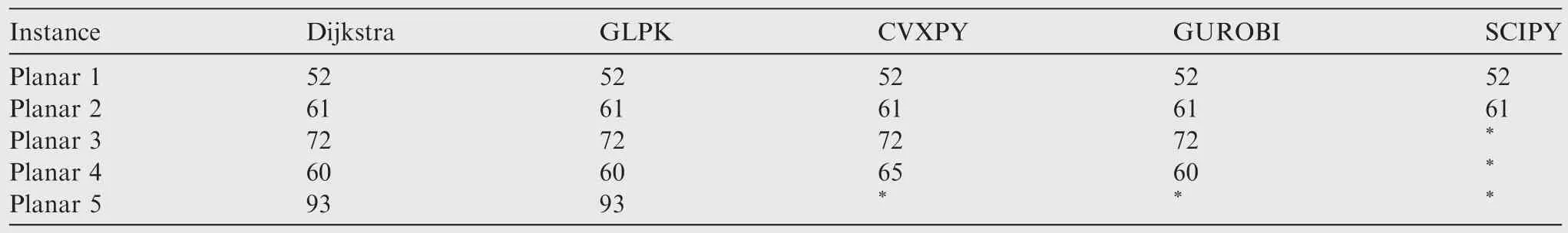
Table 14 Number of planar problem iterations with Lagrangian relaxation.

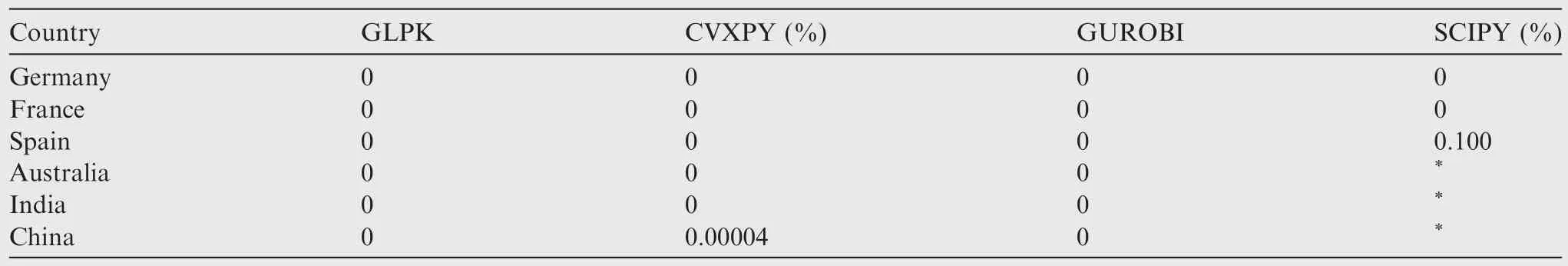
Table 15 Gaps of airport networks with column generation.

Table 16 Gaps of airport networks with Lagrangian relaxation.

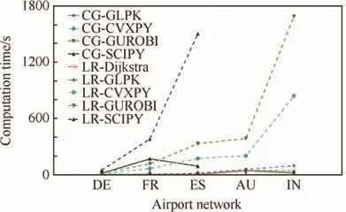
Fig.4 Comparison of computation times for airport networks.

Computation times are shown in Fig.4.The labels DE,FR,ES,AU,IN onx-axes represent the five countries Germany,France,Spain,Australia,and India.Time for solving the MCFP for the airport network of China,which is much larger than other networks,is shown in Table 17.Label*indicates that the run time is much longer than other implementations.Note that implementations of Lagrangian relaxation are slower than column generation for first five countries,but,in Table 17,the speeds of Lagrangian relaxation with Dijkstra and GLPK exceed the speed of column generation with mostof the implementations.Their performances are also close to column generation with CVXPY.

Table 17 Computation time for the airport network of China.

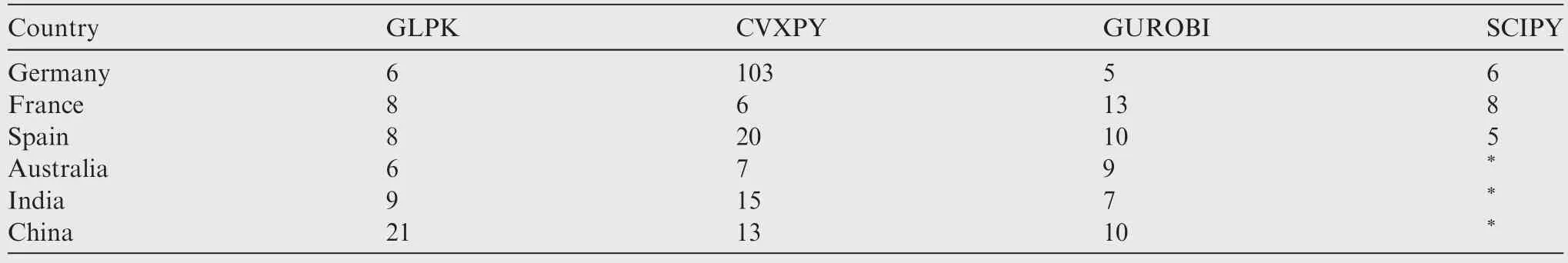
Table 18 Number of airport network iterations with column generation.

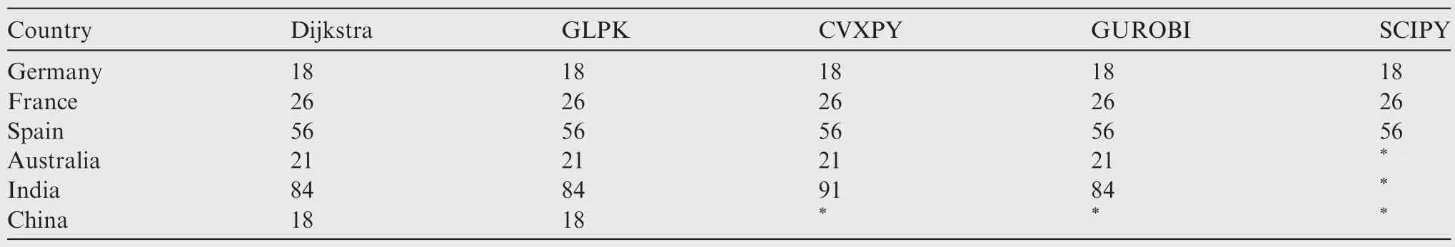
Table 19 Number of airport network iterations with Lagrangian relaxation.

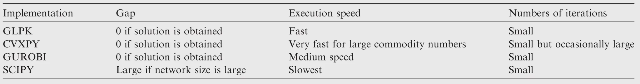
Table 20 Summary ofimplementations for column generation.

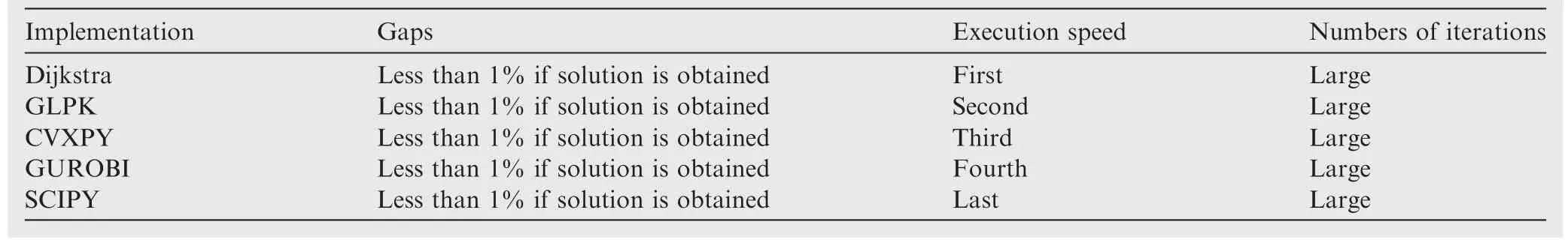
Table 21 Summary of implementations for Lagrangian relaxation.

For column generation,with the increase of network size and commodity number,the speed of CVXPY outperforms GLPK,which is the fastest implementation.CVXPY times are much shorter than GLPK for the airport network of China,as shown in Table 17.Taken together with the results of planar networks,CVXPY can have good properties while solving MCFPs with a large number of commodities.

The number of iterations are shown in Tables 18 and 19,and the result is similar to the other two groups of networks whose column generation needs less iterations.

5.4.Summary

Column generation has better properties than Lagrangian relaxation for solving MCFPs in general.However,in large networks with a high number of commodities(like the airport network of China),the best performances of Lagrangian relaxation are close with the column generation.A summary of these implementations for the two algorithms is shown in Tables 20 and 21.

6.Conclusions

In this paper,several algorithms(column generation,Lagrangian relaxation)and implementations(Dijkstra,GLPK,CVXPY,GUROBI,SCIPY)are discussed for solving multicommodity flow problems.In order to evaluate the scalability and quality of the algorithms with several implementations,three groups of networks,grid,planar and airport,are selected as case studies.

During evaluation,the objective function gaps,computation time,and numbers of iterations for different implementations are compared.It is shown that,in general,column generation performs better than Lagrangian relaxation with all the three evaluation parameters for solving MCFPs.However,for large networks with high number of commodities(like the airport network of China),Lagrangian relaxation is faster than column generation.

Separately,for column generation,GLPK has the best properties,but CVXPY can outperform GLPK while solving MCFPs with a large number of commodities.For Lagrangian relaxation,it is shown that using the Dijkstra shortest-path method to solve the Lagrangian sub-problem is the best choice.In general,GUROBI performs at a medium level in both algorithms,and SCIPY is always the worst.

This paper lays out a baseline for evaluating implementations of MCFP algorithms.For this preliminary evaluation,two algorithms and several implementations are compared.However,several other commonly-used algorithms(such as branch-and-bound)and optimization solvers are not evaluated.For future work,these solution techniques need to be considered as well,and the size of datasets should also be increased further based on the results of our study.In addition,the outcomes of this study can also be applied to certain other problems,such as different types of hub location problems.Because the performance of implementations could vary with the different scales of networks in this paper,the results for solving other problems is expected to be similar.

Acknowledgements

This study was supported by research funds from the National Natural Science Foundation of China(Nos.61521091,61650110516,61601013).

1.Sun XQ,Wandelt S,Linke F.Temporal evolution analysis of the European air transportation system:Air navigation route network and airport network.Transportmetrica B:Transp Dyn2015;3(2):153–68.

2.Ahuja RK,Magnanti TL,Orlin JB.Network flows:Theory,algorithms,and applications.Upper Saddle River:Prentice Hall;1993.p.649–94.

3.Tomlin J.Minimum-cost multicommodity network flows.Oper Res1966;14(1):45–51.

4.Barnhart C,Hane CA,Johnson EL,Sigismondi G.A column generation and partitioning approach for multi-commodity flow problems.Telecommun Syst1994;3(3):239–58.

5.Barnhart C,Hane CA,Vance PH.Using branch-and-price-andcut to solve origin-destination integer multicommodity flow problems.Oper Res2000;48(2):318–26.

6.Gondzio J,Gonzalez-Brevis P,Munari P.Large-scale optimization with the primal-dual column generation method.Math Program Comput2016;8(1):47–82.

7.Gondzio J,Gonzalez-Brevis P,Munari P.New developments in the primal dual column generation technique.Eur J Oper Res2013;224(1):41–51.

8.Gondzio J,Gonzalez-Brevis P.A new warmstarting strategy for the primal-dual column generation method.Math Program2014;152(1):1–34.

9.Karakostas G.Faster approximation schemes for fractional multicommodity flow problems.ACM Trans Algorithms2008;4(1):166–73.

10.Garg N,Konemann J.Faster and simpler algorithms for multicommodity flow and other fractional packing problems.39th Annual symposium on foundations of computer science;1998.p.300.

11.Fleischer LK.Approximating fractional multicommodity flow independent of the number of commodities.SIAM J Discr Math2000;13(4):505–20.

12.Retvari G,Biro JJ,Cinkler T.A novel lagrangian-relaxation to the minimum cost multicommodity flow problem and its application to OSPF traffic engineering.International symposium on computers and communications;2004.p.957–62.

13.Babonneau F,Vial JP.Solving large-scale linear multicommodity flow problems with an active set strategy and proximal-accpm.Oper Res2006;54(1):184–97.

14.Moradi S,Raith A,Ehrgott M.A bi-objective column generation algorithm for the multi-commodity minimum cost flow problem.Eur J Oper Res2015;244(2):369–78.

15.Bauguion PO,Ben-Ameur W,Gourdin E.A new model for multicommodity flow problems,and a strongly polynomial algorithm for single-source maximum concurrent flow.Electron Notes Discr Math2013;41:311–8.

16.Bauguion PO,Ben-Ameur W,Gourdin E.Efficient algorithms for themaximum concurrentflow problem.Networks2015;65(1):56–67.

17.Cortes P,Munuzuri J,Guadix J,Onieva L.Optimal algorithm for the demand routing problem in multicommodity flow distribution networks with diversification constraints and concave costs.Int J Prod Econ2013;146(1):313–24.

18.Zhang BW,Qi LQ,Yao EY.A multi-commodity production and distribution model in supply chain.2010 8th international confer-conference on supply chain management and information systems(SCMIS);2010 October 6–9;Hong Kong.Piscataway(NJ):IEEE Press;2011.p.1–5.

19.Caimi G,Chudak F,Fuchsberger M,Laumanns M,Zenklusen R.A new resource-constrained multicommodity flow model for conflict-free train routing and scheduling.Transport Sci2011;45(2):212–27.

20.Morabito R,de Souza MC,Vazquez M.Approximate decomposition methods for the analysis of multicommodity flow routing in generalized queuing networks.Eur J Oper Res2014;232(3):618–29.

21.Shitrit HB,Berclaz J,Fleuret F,Fua P.Multi-commodity network flow for tracking multiple people.IEEE Trans Pattern Anal Mach Intell2014;36(8):1614–27.

22.Wandelt S,Sun XQ.Efficient compression of 4D-trajectory data in air traffic management.IEEE Trans Intell Transport Syst2015;16(2):844–53.

23.Barnhart C,Krishnan N,Vance PH.Multicommodity flow problems.New York:Springer;2001.p.292–302.

24.Meng LH,Xu XH,Zhao YF.Cooperative coalition for formation flight scheduling based on incomplete information.Chin J Aeronaut2015;28(6):1747–57.

25.Jordi C,Jordi C.Improving an interior-point algorithm for multicommodity flows by quadratic regularizations.Networks2012;59(1):117–31.

26.Ye BJ,Sherry L,Chen CH,Tian Y.Comparison of alternative route selection strategies based on simulation optimization.Chin J Aeronaut2016;29(6):1749–61.

27.Gendron B,Larose M.Branch-and-price-and-cut for large-scale multicommodity capacitated fixed-charge network design.Euro J Comput Optimiz2014;2(1–2):55–75.

28.Gnu.org[Internet].Boston:GLPK–GNU Projection–Free Software Foundation,Inc.[updated 2012 June 23;cited 2017 April 28].Available from:http://www.gnu.org/software/glpk/.

29.Diamond S,Chu E,Boyd S[Internet].Berlin:CVXPY 0.4.0 Documentation,Inc.;[updated 2014 Jan 27;cited 2017 April 28].Available from http://www.cvxpy.org/en/latest/.

30.Gurobi Optimization[Internet].Houston:Gurobi Optimization–The Best Mathematical Programming Solver,Inc.;c2015-2017[updated 2017 March 22;cited 2017 April 28].Available from http://www.gurobi.com.

31.Scipy.org[Internet][updated 2017 March 18;cited 2017 April 28].Available from http://www.scipy.org.

14 June 2016;revised 8 October 2016;accepted 21 January 2017

Available online 8 June 2017

*Corresponding author at:School of Electronic and Information Engineering,Beihang University,Beijing 100083,China.

E-mail address:sunxq@buaa.edu.cn(X.SUN).

Peer review under responsibility of Editorial Committee of CJA.

Production and hosting by Elsevier

http://dx.doi.org/10.1016/j.cja.2017.05.012

1000-9361©2017 Chinese Society of Aeronautics and Astronautics.Production and hosting by Elsevier Ltd.

This is an open access article under the CC BY-NC-ND license(http://creativecommons.org/licenses/by-nc-nd/4.0/).

Multi-commodity flow problem;

Column generation;

Lagrangian relaxation;Evaluation;

Implementation