Fengjun LIU,Yifan WANG,Ying PIAO

aScience and Technology on Scramjet Laboratory,Beijing Power Machinery Institute,Beijing 100074,China

bSchool of Aerospace Engineering,Tsinghua University,Beijing 100084,China

Linear stability analysis of interactions between mixing layer and boundary layer flows

Fengjun LIUa,*,Yifan WANGb,Ying PIAOb

aScience and Technology on Scramjet Laboratory,Beijing Power Machinery Institute,Beijing 100074,China

bSchool of Aerospace Engineering,Tsinghua University,Beijing 100084,China

The linear instabilities of incompressible confluent mixing layer and boundary layer were analyzed.The mixing layers include wake,shear layer and their combination.The mean velocity profile of confluent flow is taken as a superposition of a hyperbolic and exponential function to model a mixing layer and the Blasius similarity solution for a flat plate boundary layer.The stability equation of confluent flow was solved by using the global numerical method.The unstable modes associated with both the mixing and boundary layers were identified.They are the boundary layer mode,mixing layer mode 1(nearly symmetrical mode)and mode 2(nearly anti-symmetrical mode).The interactions between the mixing layer stability and the boundary layer stability were examined.As the mixing layer approaches the boundary layer,the neutral curves of the boundary layer mode move to the upper left,the resulting critical Reynolds number decreases,and the growth rate of the most unstable mode increases.The wall tends to stabilize the mixing layer modes at low frequency.In addition,the mode switching behavior of the relative level of the spatial growth rate between the mixing layer mode 1 and mode 2 with the velocity ratio is found to occur at low frequency.

©2017 Chinese Society of Aeronautics and Astronautics.Production and hosting by Elsevier Ltd.This is an open access article under the CC BY-NC-NDlicense(http://creativecommons.org/licenses/by-nc-nd/4.0/).

1.Introduction

Linear stability of the flat plate boundary layer flow is a classical flow problem,which has been fully studied by researchers.1The numerical solution obtained via solving the Orr-Sommerfeld stability equation is useful and reliable1–3in describing the characteristics of an initial stage of boundary layer transition.The neutral curve of the flat plate boundary layer describes the stable area and the unstable area in the coordinate system formed by Reynolds number and frequency,showing the instability characteristics viewed from a linear perspective.Besides,the linear stability results can be utilized as initial-boundary conditions for direct numerical simulation or large eddy simulation in order to further study flow evolving process downstream.For instance,by forcing T-S disturbance waves solved from linear stability calculations at the inlet of a flat plate boundary layer,Joslin et al.4,5performed numerical studies on the boundary layer transition induced by subhar-monic waves and got the downstream nonlinear evolving characteristics of the subharmonics and their higher harmonics.The simulated flow transition agrees well with experimental results.Recently,some numerical transition prediction models are developed to study boundary layer transition phenomenon.6,7

Flow phenomena of mixing layers,including shear layer and wake,are very common in various fluid machineries.Same as the flat plate boundary layer flow stability problem,both shear layer and wake flow stabilities have been studied extensively and systematically.8–11For a wake flow,there exist two unstablemodes8,9which aresymmetricand antisymmetric respectively.Of these two modes,the growth rate of the symmetric mode is higher,which has been confirmed by experiments.9For a shear layer flow,there is only one unstable mode at a given disturbance frequency.10,11Taking a hyperbolic tangent function as the mean flow velocity profile for a shear layer,Michalke10studied the spatial growth characteristics of disturbance for an incompressible inviscid shear layer,and showed the variations of eigenvalues and eigenfunctions with disturbance frequency.Koochesfahani and Frieler11analyzed the linear stabilities of the mixing layer consisting of a wake and a shear layer.In their investigations,a hyperbolic tangent function and an exponential function are applied for the shear layer mean flow and the wake mean flow,respectively.The density differences of two streams are taken into consideration.If the high-density fluid is located on the lowspeed stream side,both the unstable shear layer mode and wake mode have almost the same growth rate.Otherwise the instability characteristics are similar to the mixing layer flow with uniform stream density,in which the shear layer mode is dominant.

The confluent wake and boundary layers are often observed in the multi-element airfoil with high lift.When an aircraft takes off or lands,the slat and the flap ofits airfoil move forward and backward respectively to increase lift,forming a multi-element airfoil system.When the wake generated by the slat develops downstream,it will locate above the succeeding element,or main element,and the confluent wake and boundary layer flow occur over a significant portion of the main element.The main element wake may interact with the boundary layer of the succeeding flap so as to form a confluent wake and boundary flow,too.Experiments12,13show that the confluent wake and boundary layer can exhibit entirely different behavior depending on the operation conditions such as Reynolds number and the relative position among the airfoil elements.

Except for the multi-element airfoil,the confluent mixing and boundary layers can be observed in the combustor of scramjet engines.In the duel-mode scramjet combustor,the strut14,15with fuel injection is usually employed to enhance fuel/air mixing.The shear layer at the strut trailing edge interacts with the boundary layer near the combustor chamber wall,and consequently the confluent shear layer and boundary layer flow appears.For the dual combustor ramjet16–19,the fuel-rich gas from the gas generator mixes with the supersonic air flow from the inlet,and the resulting mixing layer which contains a wake and a shear layer is restricted by the main combustor chamber wall,which leads to the confluent reacting mixing and boundary layer flow.In such a confluent flow,the combusting behavior of the mixing layer may be dramatically different from that of the mixing layer without the restriction of the chamber wall.

One author of this paper conducted the instability analysis for the incompressible and compressible confluent wake and boundary layers.20,21For the incompressible confluent flow,one instability mode associated with the boundary layer and the other instability mode associated with the wake were identified.The wake changes the shape of the boundary layer neutral curve,and the resulting critical Reynoldsnumber decreases.In addition,the wake leads to the instability mode associated with the boundary layer to be further unstable,and this instability tends to be strengthened with the velocity defect of the wake.20Therefore,the wake plays an important role in the linear development process of the boundary layer disturbance wave and the initial stage of flow transition.At high speeds,in contrast to the incompressible results,a reduced position between the wake and the boundary layer has a strong stabilizing effect on the growth rates of both the first and the second modes associated with the boundary layer.21

It should be noted that under the practical engineering application the initial mean velocity profile for a mixing layer almost has not only a wake component due to the boundary layers on the two sides of the splitter plate,but also a shear layer component due to the velocity difference of the two streams.Such a mixing layer containing a wake and a shear layer interacts with a boundary layer and forms the confluent mixing and boundary layer flow,which is taken into consideration in the present paper.The linear stability theory is used to study the instability of the confluent flow,with the focus on the flow stability interactions between the mixing layer and the boundary layer.The confluent mean flow model is the direct superposition of the Blasius boundary layer flow and the mixing layer flow,where a hyperbolic tangent function is chosen for the shear layer and an exponential function is chosen for the wake.The disturbance amplitude of the confluent flow is assumed to be small enough so that it can be described by the Orr-Sommerfeld stability equation.The central differential scheme with the sixth order accuracy is used to discretize the stability equation and the resulting discretization equation is solved using the global numerical method.The whole eigenvalue spectrum including the discrete and continuous part is obtained.The instability modes associated with the boundary layer and the mixing layer are identified.The effects of the critical gasdynamic and geometric parameters on those instability modes are analyzed and the instability characteristics of the confluent flow are obtained.

The confluent mixing and boundary layer flow model is given in the following section and then the Orr–Sommerfeld equation is briefly derived.It is followed by the global numerical method,discussion for the confluent flow stability analyses and concluding remarks.

2.Confluent flow model

The confluent flow considered here consists of a flat plate boundary layer and a mixing layer which is located a certain distance away from the flat plate.The mean velocity profile of the confluent flow is the superposition of that of the boundary layer and that of the mixing layer.

Fig.1 shows the mean velocity profile of the confluent flow,whereUis the non-dimensional velocity andyis the nondimensional normal distance away from the wall.The reference velocity isU∞,the velocity at the edge of the boundary layer,and the reference length is the boundary layer displacement thickness δ*.wis the wake depth indicating the velocity defect andhis the mixing layer height which is the distance between the mixing layer and the wall.Except for the mean velocity profile of the confluent mixing layer(wake+shear layer)and boundary layer(WSBL)flow,those of the confluent wake and boundary layer(WBL)flow and the confluent shear layer and boundary layer(SBL)flow are shown in Fig.1 for comparison.

The confluent flows mentioned above are assumed to be parallel,in which the streamwise velocity component varies only along the normal wall,and the normal velocity component and the spanwsie velocity component are zero.The mean velocity profile of the boundary layer is obtained by solving the Blasius boundary layer similarity equation.For the wake and the shear layer flows,the mean velocity profiles are taken as the exponential function9and the hyperbolic tangent function10,11receptively.As a consequence,the superposed profile of the confluent mixing and boundary layer flow is given as

whereU(y)B.L.represents the mean velocity profile of the boundary layer,andka parameter for changingU2/U1,the velocity ratio of the shear layer.

3.Stability equation and numerical method

In Cartesian coordinate system(x*,y*,z*,t*),t*denotes time.x*,y*andz*represent the streamwise,wall normal and spanwise direction respectively and the corresponding instantaneous velocity components areu*(x*,y*,z*,t*),v*(x*,y*,z*,t*)andw*(x*,y*,z*,t*)respectively.The confluent mixing and boundary layer flow can be decomposed into the mean flow which is steady and the superposed disturbance flow which is unsteady.The instantaneous flow variables thus have the following expressions:where the variables with a prime denote fluctuation component,and the upper case denotes the mean flow variable.HereU*denotes velocity,P*denotes pressure.

For simplicity,the parallel flow assumption,commonly used in hydrodynamic stability analyses,is applied.This approximation results in the leading-order problem in a multiple scale method that includes the effects of the slow flow divergence.22Thus,in the current analysis,the nonparallel effects are not considered.The continuity and the momentum equations are nondimensionalized with respect to the velocity at the edge of the boundary layerU∞,the kinematic viscosity υ and the displacement thickness of the boundary layer δ*.A Reynolds number can then be defined asRe=U∞δ*/υ.

Substituting Eq.(2)into the incompressible Navier–Stokes equations,omitting the second order or higher fluctuation terms and eliminating the pressure term,the linearized equation for cross-stream fluctuation velocity can be derived as

Disturbances are assumed to be traveling waves and separable solutions are then sought for the fluctuating velocity componentv'in the non-dimensional form:

where α is the streamwise wave number with a form of complex number,i.e.α = αr+iαi,ω the disturbance frequency,and(y)the eigenfunction of the fluctuating velocity componentv'.

By substitution of Eq.(4)into Eq.(3),the Orr-Sommerfeld stability equation can be obtained as

Eq.(5)governs the mode shape of wavelike disturbances associated with the base profile in terms of the streamwise wave number α,the wave frequency ω and the Reynolds numberRe.The boundary conditions for(y)are

The global numerical method23is used to solve the stability equation.The spectral method based on Chebyshev series and the finite difference method may be used to discretize the stability Eq.(5).Although the former is of high accuracy,the mesh at both boundary layer and mixing layer of the confluent flow needs to be clustered and it thus is hard to be applied due to the difficulty of finding an analytical mapping transformation between the spectral domain and the physical domain.As a consequence,the central difference scheme with the sixth order accuracy is employed to discretize Eq.(5)and the resulting equation is given by

where the subscript ‘n” stands for the grid points,and C the coefficient matrix independent of the wave number α.

The eigenvalue problem of Eq.(7)is nonlinear and of order four in the eigenvalue α,and various approaches are available to solve such a problem.The global method giving the discrete spectrum of eigenvalues without a prior knowledge of the value is employed in the present paper.

The application of the boundary conditions to Eq.(7)causes those coefficient matrices to be singular.The algebraic eigenvalue transformation to remove the singularities is given by

Eq.(7)with the application of the eigenvalue shift becomes

The matrices with the tilde are nonsingular.

The linear companion matrix method is used to linearize the nonlinear problem and the linearization yields

where I is the identity matrix of ordernandthe identity matrix of order 4n.Eq.(10)can be further transformed to an algebraic eigenvalue problem seeking the eigenvalues of matrix A

The eigenvalues are found from Eq.(11)by using the QR or QZ algorithm.

Upon the obtained eigenvalues,the eigenfunctions may effectively be found by the inverse iteration formula24

where σ is a normalizing factor.The procedure converges in two or three iterations for an initial guess of(v0)T=[1,1,...,1]T.

4.Presentation of results

In order to validate the current numerical solver,the eigenvalues for the Blasius boundary layer flow,the shear layer flow and the wake flow are calculated.Fig.2 shows a comparison of calculated neutral curve with that of Jordinson3for the Blasius boundary layer and the well overlapping curve can be seen.

Fig.3 compares the calculated streamwise wave number α = αr+iαiwith that of Michalke10for a shear layer flow.The same hyperbolic tangent function is taken as the mean flow velocity profile.The present real and imaginary parts of the wave number with different disturbance frequency ω are in well agreement.

Table 1 shows the calculated wave number with three downstream distancesx/Lfor a wake flow and the comparison with that of Mattingly and Criminale.9The wake defect decreases gradually with downstream distance,and the unstable wave growth rate of both symmetrical mode(also known as mode 1)and anti-symmetrical mode(also known as mode 2)decreases correspondingly.The present numerical solver correctly predicts the stability development trend and the data agree well with those from Mattingly and Criminale.9

It can be seen from the above comparisons that the present solver is able to accurately predict the stability characteristics of the boundary layer,shear layer and wake flows.For the confluent mixing layer(containing shear layer and wake)and boundary layer flow,the stability governing equation and boundary conditions are exactly the same as those of the isolated boundary layer,shear layer or wake flow.As a result,the current numerical solver should be capable of analyzing the confluent flow instabilities.

Fig.4 shows the spectra of the wave speed for the confluent mixing and boundary layers,in which the horizontal and longitudinal coordinates respectively represent the real and imaginary parts of the wave speedC= ω/α=Cr+iCi,withRe=900 and ω=0.0984.The velocity ratio of shear layerU2/U1=0.4,the mixing layer heighthis 10,and the wake depthwis 0.5.The computational grid is clustered both in the boundary layer and mixing layer to ensure enough grid points there.The wave speed spectra for the isolated Blasius boundary layer with the same related parameters are also included for comparison.

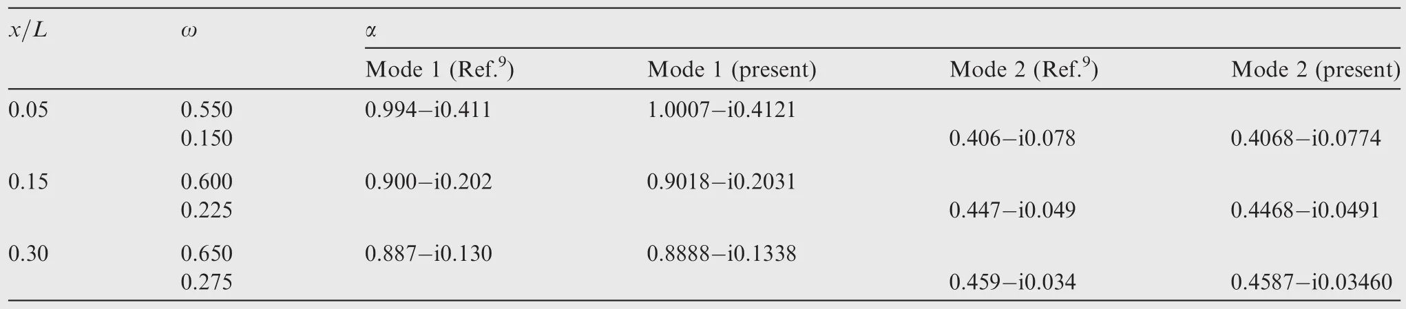
Table 1 Calculated wave number α for a wake flow.

The flow stability studies for the mixing layer consisting of a shear layer and a wake show11that two unstable modes have been identified,with one mode dominated by the symmetrical disturbance shape and the other by the anti-symmetrical shape.It can be seen from Fig.4 that three discrete unstable modes appear in the confluent flow.One mode is identified as the boundary layer mode due to its coincidence with the boundary layer mode alone,and the growth rate and disturbance shape of the other two modes are similar to those of Koochesfahani and Frieler11,whose eigenvalues are very close to those of the mixing layer mode 1(nearly symmetrical mode)and mode 2(nearly anti-symmetrical mode)respectively.Then they can be identified as the mixing layer modes 1 and 2 respectively by further checking their eigenfunctions.

For the grid independent study,the stability characteristics of the confluent mixing and boundary layer flow have been calculated using five grids with the grid point number of 61,81,101,121 and 141,all of which are refined in the areas of the boundary layer and the mixing layer.Table 2 shows the variations of the wave number α with grid point number,with the mixing layer heighth=7.5,Re=998, ω=0.1122,U2/U1=0.4 and the wake widthw=0.5.It can be seen that the calculated wave numbers remain unchanged when the grid number is over 121,which is used for all the stability calculations for the confluent flow.

Fig.5 shows the neutral curves of the boundary layer mode for three confluent flows including SBL,WBL and WSBL,withh=7.5,U2/U1=0.4 andw=0.5.The neutral curve for the Blasius boundary layer(BL)is also included for comparison.

It can be found that the neutral curves move to the upper left due to the presence of the shear layer or the wake or the mixing layer,with the largest movement extent occurring in the lower branch for the WSBL.The resulting critical Reynolds numbers for the present case decrease,with 481 for the WBL,492 for the SBL and 497 for the WSBL.The disturbance frequencies at which the critical Reynolds numbers appear for all the confluent flows increase slightly.

Fig.6 shows the changes of the growth rate for the boundary layer mode for the three confluent flows with frequency and Reynoldsnumber,withh=7.5,U2/U1=0.4andw=0.5.The T-S wave growth rate of the Blasius boundary layer is also included for comparison.

It can be seen from Fig.6 that the growth rate of the most unstable mode for the confluent flows tends to increase,and the increasing amplitude is larger at the low Reynolds number ofRe=600,with the largest amplitude of 50.5%appearing in the case of WBL.Besides,the frequency corresponding to the most unstable mode for all the confluent flows tends to increase as well,among which that of the WSBL has the largest increasing amplitude of 4.7%.

Fig.6 also shows that at the low Reynolds number ofRe=600 the unstable boundary layer modes in both the WBL and the SBL are further destabilized and the unstablefrequency zones are broadened.For the WSBL,the neutral frequencies increase in both the lower and upper branches,and the mixing layer has a destabilized or stabilized effect on the boundary layer mode depending upon frequency.In the present case,the unstable boundary layer mode is stabilized when frequency is lower than 0.1054,and vice versa.The frequency zone in which the boundary layer mode is destabilized is obviously broader than that stabilized.At high Reynolds number ofRe=1200,the stability feature of the boundary layer mode in the WBL and SBL resembles that in the WSBL,with the neutral frequency increasing in the two branches.

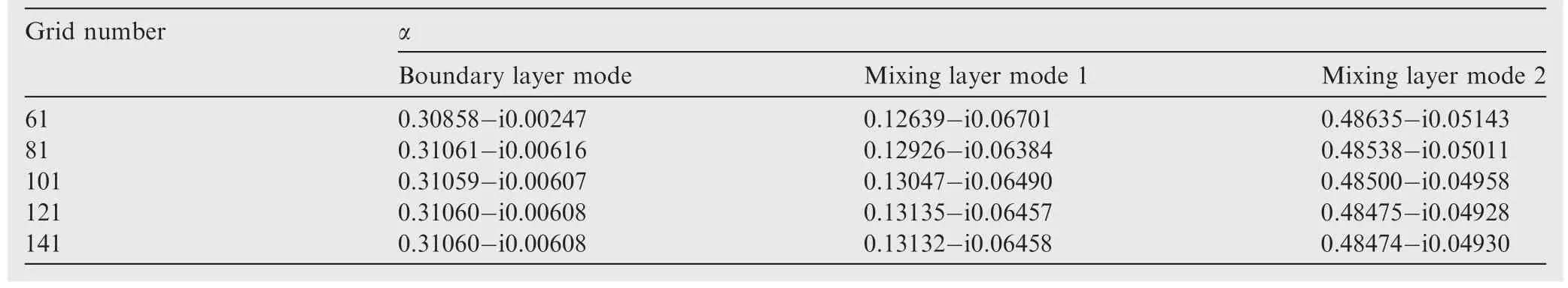
Table 2 Effect of grid number on wave number α for confluent flow.

In general,the growth rate of the most unstable boundary layer mode increases and the corresponding frequency decreases with Reynolds number.As can be seen from Fig.7,which shows the variation of the growth rate of the most unstable boundary layer mode with Reynolds number,the most unstable modes associated with the boundary layer in the confluent flows are further destabilized compared to the isolated boundary layer,with the most destabilized case appearing in the WBL.The frequency corresponding to the most unstable mode becomes higher,with the highest case appearing in the WSBL,as shown in Fig.8.

Fig.9 shows the change in the growth rate of the most unstable boundary layer mode for the WSBL with the mixing layer height and the velocity ratio,withRe=900 andw=0.5.The result for the isolated boundary layer is also included for comparison.It can be seen that the reduced mixing layer height has an amplified effect on the most unstable boundary layer mode,and this stability feature becomes more prominent with the velocity ratio.

Fig.10 shows the unstable frequency spectra for the mixing layer modes for the WSBL and the isolated mixing layer(containing wake and shear layer,WSL),with velocity ratioU2/U1=0.4,U2/U1=0.8,Re=900,w=0.5 andh=7.5.When the mixing layer is brought close to the wall,the unstable mixing layer modes are stabilized in the low frequency zone before the most unstable mode appears,particularly for the mixing layer mode 1,while in the high frequency zone nearly after the most unstable mode appears,the boundary layer has no effect on the stability of the mixing layer.

Fig.10 also shows a switching behavior of the relative level of the spatial growth rate between the mixing layer modes 1 and 2.For the velocity ratioU2/U1=0.4,the mode 2 is more unstable than the mode 1 in the lower frequency zone while the mode 1 tends to be more unstable than the mode 2 for any frequency for the velocity ratioU2/U1=0.8.The effect of the velocity ratio on the unstable mixing layer modes 1 and 2 is given in Fig.11,further showing the switching behavior that occurs atU2/U1≈0.55 in the present case.

Fig.12 shows the effect of the velocity ratio on the frequency spectra for the mixing layer modes,withRe=900,h=7.5,w=0.5.As the velocity ratio increases,the frequency range of the unstable mixing layer modes 1 and 2 becomes wider,while the growth rate of the most unstable modes decreases.

Fig.13 shows the effect of the mixing layer height on the unstable mixing layer mode 1,withRe=900,ω=0.1,w=0.5.At this frequency,the unstable mixing layer modes are stabilized with the reduced mixing layer height,as also shown in Fig.10.When the mixing layer height is over 20,the stability of the mixing layer mode 1 is no longer affected by the wall.

5.Conclusions

The linear spatial stability analyses for the incompressible confluent shear layer and boundary layer(SBL),wake and boundary layer(WBL)and mixing layer(containing a wake and a shear layer)/boundary layer(WSBL) flows have been carried out using the linear stability theory,with the focus on the last that is of more interest in the practical engineering application.The global numerical method is used to solve the stability equation describing the con fluent flow.The unstable modes have been identified for all the three con fluent flows.For the WSBL,the identified unstable modes are the boundary layer mode,the mixing layer mode 1(nearly symmetrical mode)and the mixing layer mode 2(nearly anti-symmetrical mode).

The neutral curves of the boundarylayer modein the con fluent flows move to the upper left and the critical Reynolds number decreases.Compared to 520 for the Blasius boundary layer,the values for the WBL,SBL andWSBL are 481,492 and 497 in the present case,respectively.When the mixing layer is brought v can be destabilized or stabilized,depending on frequency.And the high frequency range in which the destabilized mode appears is wider than the low frequency range stabilized.Unlike the WSBL,the unstable boundary layer mode in the WBL and SBL can be completely destabilized in the entire unstable frequency range at low Reynolds number.In addition,the growth rate of the most unstable boundary layer mode is further amplified in all the three con fluent flows.

When the mixing layer is far away enough from the wall,such as 20 times the displacement thickness of the boundary layer or higher,the interaction between the mixing layer and the boundary layer is slight and their stabilities are not affected by each other.The wall has a damping effect on the unstable mixing layer modes with the reduced mixing layer height,which only occurs in the low frequency zone nearly before the most unstable mode appears.The damping of the mixing layer mode 1 is obviously more than the mixing layer mode 2.Moreover,switching behavior of the relative level of the spatial growth rate between the mixing layer modes 1 and 2 is found to occur for the low frequency with the velocity ratio.

Acknowledgement

This study was supported by the National Natural Science Foundation of China(No.51476152).

1.Schlichting H.Boundary layer theory.New York:McGraw-Hill;1951.

2.Mack LM.Boundary-layer linear stability theoryCourse on stability and transition of laminar flow.Paris:AGARD;1984.

3.Jordinson R.The flat boundary layer.Part 1:Numerical integration of the Orr-Sommerfeld equation.J Fluid Mech1970;43(4):801–11.

4.Joslin RD,Streett CL,Chang CL.Spatial direct numerical simulation of boundary-layer transition mechanisms:Validation of PSE theory.Theor Comput Fluid Dyn1993;4(6):271–88.

5.Joslin RD,Streett CL.The role of stationary cross-flow vortices in boundary layer transition on swept wings.Phys Fluids1994;6(10):3442–53.

6.Xia CC,Chen WF.Boundary-layer transition prediction using a simplified correlation-based model.Chin J Aeronaut2016;29(1):66–75.

7.Xu JK,Bai JQ,Zhang Y,Qiao L.Transition study of 3D aerodynamic configures using improved transport equations modeling.Chin J Aeronaut2016;29(4):874–81.

8.Sato H,Kuriki K.The mechanism of transition in the wake of a thin flat plate placed parallel to a uniform flow.J Fluid Mech1961;11(3):321–52.

9.Mattingly GE,Criminale WO.The stability of an incompressible two-dimensional wake.J Fluid Mech1972;51(2):233–72.

10.Michalke A.On spatially growing disturbances in an inviscid shear layer.J Fluid Mech1965;23(3):521–44.

11.Koochesfahani MM,Frieler CE.Inviscid instability characteristics offree shear layers with non-uniform densityAIAA 25th aerospace sciences meeting.Reston(VA):AIAA;1987.

12.Krumbein A.On modeling of transitional flow and its application on a high lift multi-element airfoil configuration41st AIAA aerospace sciences meeting and exhibit;2003 January 6–9;Reno,Nevada,USA.Reston(VA):AIAA;2003.

13.Rumsey CL,Lee-Rasusch EM,Watson RD.Three-dimensional effects on multi-element high lift computations.Reston:AIAA;2002,Report No.:AIAA-2002-0845.

14.Rust B,Gerlinger P,Lourier JM,Kindler M,Aigner M.Numerical simulation of the internal and external flowfields of a scramjet fuel strut injector including conjugate heat transfer.Reston(VA):AIAA;2001,Report No.:AIAA-2011-2207.

15.Sato S,Munakata T,Fukui M.Application of 3-dimensional effects of shock waves caused by a strut-cowl system in a scramjet engine.Reston(VA):AIAA;2011,Report No.:AIAA-2011-2314.

16.Billig FS,Waltrup PJ,Stockbridge RD.Integral-rocket dualcombustion ramjets:A new propulsion concept.J Spacecraft Rockets1980;17(5):416–24.

17.Mercier R,McClinton C.Hypersonic propulsion–transforming the future offlight.Reston(VA):AIAA;2003,Report No.:AIAA-2003-2732.

18.Foelsche RO,Leylegian JC,Betti AA,Chue RSM,Marconi F,Beckel SA,et al.Progress on the development of a freeflight atmospheric scramjet test technique.Reston(VA):AIAA;2005,Report No.:AIAA-2005-3297.

19.Ahn J,Starkey RP.Application of evidence theory on dual combustor ramjet model.Reston(VA):AIAA;2013,Report No.:AIAA-2013-3752.

20.Liou WW,Liu FJ.Spatial linear instability of confluent wake/boundary layers.AIAA J2001;39(11):2076–81.

21.Liou WW,Liu FJ.Compressible linear stability of confluent wake/boundary layers.AIAA J2003;41(12):2349–56.

22.Morris PJ.Stability of a two-dimensional jet.AIAA J1981;19(7):857–62.

23.Bridges TJ,Morris PJ.Differential eigenvalue problems in which the parameter appears nonlinearly.J Comput Phys1984;55(3):437–60.

24.Joslin RD,Streett CL,Chang CL.Validation of three-dimensional incompressible spatial direct numerical simulation code:A comparison with linear stability and parabolic stability equation theories for boundary-layertransitiononaflatplate.Washington,D.C.:NASA;1992,Report No.:NASA-TP-3205.

6 June 2016;revised 14 September 2016;accepted 28 September 2016

Available online 14 June 2017

*Corresponding author.

E-mail address:liu8024@126.com(F.LIU).

Peer review under responsibility of Editorial Committee of CJA.

Production and hosting by Elsevier

http://dx.doi.org/10.1016/j.cja.2017.04.011

1000-9361©2017 Chinese Society of Aeronautics and Astronautics.Production and hosting by Elsevier Ltd.

This is an open access article under the CC BY-NC-ND license(http://creativecommons.org/licenses/by-nc-nd/4.0/).

Boundary layer;

Flow instability;

Linear stability theory;

Shear layer;

Wake