Alejandro MURRIETA-MENDOZA,Bruce BEUZE,Laurane TERNISIEN,Ruxandra Mihaela BOTEZ

Research Laboratory in Active Control,Avionics,and Aeroservoelasticity(LARCASE),Universite´du Que´bec(E´cole de Technologie Supe´rieure–E´TS),Montreal H3C 1K3,Canada

New reference trajectory optimization algorithm for a flight management system inspired in beam search

Alejandro MURRIETA-MENDOZA,Bruce BEUZE,Laurane TERNISIEN,Ruxandra Mihaela BOTEZ*

Research Laboratory in Active Control,Avionics,and Aeroservoelasticity(LARCASE),Universite´du Que´bec(E´cole de Technologie Supe´rieure–E´TS),Montreal H3C 1K3,Canada

With the objective of reducing the flight cost and the amount of polluting emissions released in the atmosphere,a new optimization algorithm considering the climb,cruise and descent phases is presented for the reference vertical flight trajectory.The selection of the reference vertical navigation speeds and altitudes was solved as a discrete combinatory problem by means of a graphtree passing through nodes using the beam search optimization technique.To achieve a compromise between the execution time and the algorithm’s ability to find the global optimal solution,a heuristic methodology introducing a parameter called ‘optimism coefficient was used in order to estimate the trajectory’s flight cost at every node.The optimal trajectory cost obtained with the developed algorithm was compared with the cost of the optimal trajectory provided by a commercial flight management system(FMS).The global optimal solution was validated against an exhaustive search algorithm(ESA),other than the proposed algorithm.The developed algorithm takes into account weather effects,step climbs during cruise and air traffic management constraints such as constant altitude segments,constant cruise Mach,and a pre-defined reference lateral navigation route.The aircraft fuel burn was computed using a numerical performance model which was created and validated using flight test experimental data.

©2017 Chinese Society of Aeronautics and Astronautics.Production and hosting by Elsevier Ltd.This is an open access article under the CC BY-NC-NDlicense(http://creativecommons.org/licenses/by-nc-nd/4.0/).

1.Introduction

Several studies by aeronautical authorities and associations have estimated that the number of aircraft in service will increase in the forthcoming years.1Having more aircraft airborne will bring new challenges to air traffic management to guarantee safe and efficient flights.

Worldwide,several programs have been initiated for the research,developmentand implementation ofsystems,regulations and procedures for future air traffic management.These programs include the Next Generation Air Transport System(NextGen)in North America,led by the United States,the Single European Sky Air Traffic Management(ATM)Research(SESAR)in Europe,and the Collaborative Actions for Renovation of Air Traffic Systems(CARATS)in Japan.These programs improve ATM to guarantee safety,expand air space capacity,reduce polluting emissions,and to provide flight trajectories as efficient as possible.

Efficient flight reference trajectories result in both flight time and fuel burn reductions.Flying these trajectories is extremely desirable,since fuel burn reduction directly diminishes polluting emissions,as well as saved on costs.As pointed out by the Air Transport Action Group(ATAG),around 2%of the carbon dioxide(CO2)emissions released to the atmosphere are caused by aeronautical activities.2The industry has set itself the goal of reducing its CO2emissions to 50%of those generated in 2005 by 2050.3Many organizations have been created to address and solve the pollution problems.One such example is the Business-led Network of Centers of Excellence Green Aviation Researchamp;Development Network(GARDN)in Canada,which encourages services and products to reduce polluting emissions.

Several new technologies and aircraft modifications have already been considered with the aim to reduce polluting emissions in which winglets have been proven to improve aircraft efficiency.4What’s more,changes in materials and avionics equipment have reduced aircraft weight,as well as the introduction of biofuels,5and engine improvements have also reduced fuel burn.Airlines can achieve fuel savings with their current fleets by implementing different operational measures,such as the single engine taxiing,ground power units,engine washing,and flight reference trajectory optimization as presented in Ref.6 Therefore,implementing these improvements in current fleets is becoming a necessity,since the newer aircraft generations alone will not be enough to fulfill the industry’s polluting reduction goals.7

The Continuous Descent Approach(CDA),an operational procedure related to flight reference trajectory optimization,has been proven to reduce fuel consumption.With this procedure,the aircraft descends with the engines in the IDLE mode(least fuel consuming setting)instead of descending in the conventional step descent pattern.Several airports have implemented this technique because it contributes to fuel savings and noise reduction.8–11The CDA must be implemented correctly to avoid the need to execute a missed approach procedure,which is expensive in terms offuel burn and pollution emission release.12,13Other approaches,such as air to air refueling was studied in Ref.14 and aircraft ground movement optimization was suggested in.15

For ‘en-route” operations,Jensen et al.16,17in stated that aircrafts in the United States do not fly at their optimal speed or altitude.Other discussions have been conducted regarding the savings that flying at low cruise speeds may bring,as well as at how lower cruise speeds would affect other aircraft flying near the low-speed cruise aircraft.18,19Turgut et al.20developed equations to obtain the fuel flow for different aircrafts and found out that flight trajectories for national flight within Turkey can be improved.

Current reference trajectory optimization was done by ground teams or by airborne avionics such as the commercial Flight Management System(FMS).The former can use algorithms that require many computational resources to find the optimal reference trajectory;the latter require fast algorithms to find an optimal or a sub-optimal reference trajectory.

The reference trajectory could be studied in two different dimensions:The vertical dimension and the lateral dimension.The first consists in the speeds and altitudes that provide the most economical flights,and the latter consists in the geographical waypoints where no obstacles are present,and where the aircraft can take advantage of weather,such as tail winds,to reduce the flight cost.

A number of optimization algorithms have been implemented to solve the reference trajectory optimization problems.Different optimal control techniques considered various constraints and optimization objectives.21–27Equations of Motion(EoM)were used in these optimal control based algorithms in order to find the optimal solution.Other authors applied the dynamic programming;such as Yoshikazu et al.28who developed a moving search space algorithm by taking into account both weather and the Required Time of Arrival(RTA)constraints.Ng et al.29also used dynamic programming,by taking into account winds for a fixed Mach number and by allowing changes in the flight level during the cruise regime.Hagelauer and Mora-Camino30utilized the EoM to implement dynamic programming with neural networks to optimize trajectories,underscoring the fact that FMSs use numerical performance databases instead of EoM.

In Reference trajectory optimization focusing on avoidance(obstacles or weather constraints)has also been investigated.Cobano et al.31applied the Particle Swarm Optimization(PSO)for a 4D(RTA constraint considered)trajectory.Ripper et al.32used graph search algorithms to optimize the route of a general aviation aircraft while avoiding obstacles.The dynamic physical principles of a stream avoiding obstacles were adapted to the path trajectory optimization.This methodology allowed the avoidance of objects of different shapes.33An algorithm able to optimize the flight trajectory of cooperative Unmanned Aerial Vehicles(UAV)able to avoid obstacles was developed using a combination of the central force optimization algorithm and genetic algorithms in Ref.34.

All these optimization algorithms were able to optimize the flight reference trajectory by fulfilling their imposed constraints.However,solving the EoM to find the optimal trajectory in a system with limited processing power,such as an FMS,can be very much time consuming,leading its implementation to be impractical.Therefore,the FMS do not normally use these equations,and instead use a set of look up tables with experimental data called a numerical performance model.

Numerical performance models provide fuel consumption information,and therefore researchers have developed fuel burn estimators that work with this type of models to compute the cost of a cruise segment.35These estimators were later used to optimize flights in cruise.36Fe´lix et al.37used genetic algorithms to find the optimal trajectory by taking advantage of winds.Murrieta and Botez38used the Dijkstra’s algorithm to find the optimal trajectory by taking advantage of winds and temperatures.

The vertical reference trajectory optimization problem applied on a numerical performance model for all flight phases can be treated as a combinatorial problem.The number of possible solutions(feasible or not)are defined by combinations of Indicated Air Speeds(IAS),Mach numbers and altitudes available in the numerical performance model.Although the number of combinations for evaluation available in the numerical performance model might be considered low compared against the number of combinations available in classical optimization problems(e.g.the Traveling Salesman Problem(TSP),where a salesmen at a given origin city should visit every available city at least once and he must return to the origin city,is a hard Nondeterministic Polynomial(NP)time problem.For a high number of cities,there is no practical optimization solution able to guarantee optimality),it should be taken into account that the FMS possesses low power computation capabilities.Just a small part of these computation capabilities are dedicated to the reference trajectory optimization,as other critical operations have higher priority39such as to provide the current trajectory guidance,to monitor the aircraft flight envelope so as to guarantee a safe flight,to control automatically the engine thrust,and etcetera.In a real time environment,systems such as the FMS,should be able to provide solutions(either ‘optimal” or good ‘sub-optimal”)in a short period.

To solve this optimization problem for an FMS,Gagne´et al.40developed a space reduction search algorithm.Murrieta and Botez41developed an optimization algorithm by reducing the space search even further and thus the execution time.Fe´lix et al.42used a numerical performance database and the golden section search algorithm to find the climb speed schedule and the Top of Climb(ToC)altitude in order to optimize a short flight,and to implement step climbs in long haul flights.

Coupling and optimizing the lateral and the vertical reference profiles has also been a promising research area.Murrieta43proposed five different reference lateral trajectories to be evaluated using a previously computed optimal vertical reference trajectory.Fe´lix et al.44implemented genetic algorithms to optimize the vertical reference trajectory.Felix et al.45,46used genetic algorithms to simultaneously optimize the lateral and vertical reference trajectories for the cruise phase.Genetic algorithms provided good solutions,however their metaheuristic nature made them difficult to certify,and thus implemented in current airborne avionics.

In this paper,the vertical reference trajectory optimization problem is solved with the Beam Search Algorithm(BSA).The implementation of this algorithm to the reference trajectory problem has not yet been studied in the literature.Beam search is a deterministic algorithm which requires low memory(the decision tree is reduced).This algorithm can quickly provide good solutions,even if they are not the optimal ones.All these characteristics are desirable for the FMS.

The algorithm proposed in this paper,compared with the above mentioned algorithms used for the vertical reference trajectory optimization by using numerical performance models,brings the novelty of treating this problem in a ‘decision tree”.The speeds and altitudes in the numerical performance model are discrete values.The Beam Search Algorithm,unexplored for this problem,has been adapted to the vertical trajectory problem to explore its optimization capabilities.This paper also introduces a new heuristic(technique used to provide an approximate solution to a problem in a reasonable time)used by the algorithm to estimate the flight cost at any node within the decision tree.This heuristic takes into account all flight phases,weather conditions,step climbs,and is designed to be used in a numerical performance model.

The algorithm developed in this paper takes into account winds,temperature and current traffic control constraints such as the constant speed and the constant flight level.Changes in the flight level(step climbs)during cruise are evaluated at a pre-defined time frame to mimic the cruise-climb regime.Since this algorithm was developed with the goal of being implemented in current and future FMS generations,a numerical performance model was used instead of the EoM.

The paper is organized as follows:Section 1 defines the performance database used to compute flight costs;Section 2 offers a brief explanation of how a flight cost is computed using a performance numerical model;The BSA is briefly explained,and its implementation is fully explained in detail in Section 3;Section 4 presents and discusses the results;and the conclusions are provided in the last section.

2.Methodology

2.1.Numerical performance model

The numerical performance model is a set of tables containing an aircraft’s performance in different flight phases.The available flight phases are provided in Table 1.This numerical performance model is developed and validated using experimental flight test data.It replaces the conventional EoM widely usedin the literature.This model is fairly expensive to be created with experimental flight data,and an alternative is to use a Level D research flight simulator.47

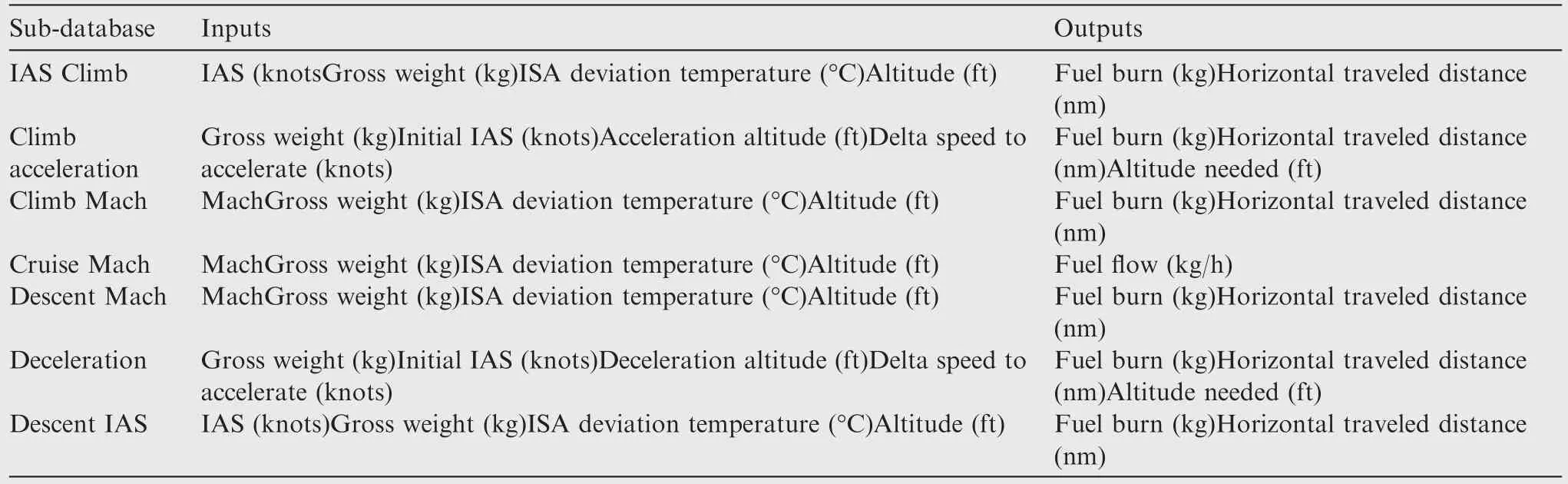
Table 1 Numerical performance model sub-databases.

The inputs in the numerical performance model are provided as discrete values.For example,for the IAS climb sub-database,the IAS input is provided in 10 knots(1 knots=1.852 km/h)separations,as shown in Eq.(1),(1 ft=0.3048 mm)wherenis the last available IAS.

2.2.Flight cost computation

The flight cost computations for the vertical reference trajectory were performed using the method described in Ref.48 In this method,climb in IAS,climb in Mach number,acceleration,cruise,descent in Mach number,deceleration and descent in IAS are taken into account by considering the particularities of each phase,such as ‘crossover altitudes”,‘step-climbs”,etc.A brief explanation of this method is given here for completeness.

By providing the input vector given by Eq.(2),along with a takeoff weight,a cost index and a reference lateral route,the method computes the fuel burn,the flight time and the flight cost.These parameters are accumulated in two different variables called Fuel Burn(kg)and Flight Time(h),respectively.Eq.(3)is used for computing the trajectory reference flight cost.

where Cost Index(kg/h)is a parameter that relates time to cost in fuel terms.The Cost Index is normally de fined by airlines before take-off and considers crew,maintenance and other time-related costs.A high Cost Index value makes the aircraft fly at higher speeds in order to reduce Flight Time even if these speeds are not efficient in terms offuel burn.This is because Flight Time has a strong in fluence on Eq.(3).A low cost index value diminishes the importance of Flight Time in Global Cost,thus the algorithm focuses mostly on reducing the fuel burn.The aircraft can fly at lower speeds if they are more efficient in terms of fuel burn.

The altitudes and speeds considered to compute the flight cost are only those available in the numerical performance model.However,the aircraft‘s gross weight constantly changes as fuel is burned,and the International Standard Atmosphere(ISA)deviation temperature changes while the aircraft is in flight.Weight and ISA deviation temperature deviations can take values that are not exactly those available in the discrete numerical performance model input values.

For this reason,a series of linear Lagrange interpolations were executed using the numerical performance models limits to compute the fuel burned and the horizontal traveled distance.During climb and descent,interpolations were performed at altitudes multiples of 1000 ft.During the cruise regime,interpolations were executed every 25 nautical miles for the current aircraft weight and the local ISA deviation temperature.This method takes into account the step climb costs as well as weather conditions.The possibility of executing step climbs is evaluated every hour of flight.Weather information is obtained from forecasts provided by Environment Canada.A typical vertical flight profile is shown in Fig.1.

Throughout the paper,when this interpolations method is used,it is referred to as ‘real cost computation”.This method has the particularity that is time consuming,so it should be executed as few times as possible.

3.Optimization algorithm

3.1.Space search:Decision graph

The decision variables for the vertical reference trajectory optimization problem are the IAS climb,the IAS descent,the Mach number and the cruise altitude.Since the decision variables can take only the pre-defined values in the numerical performance model, the problem becomes a ‘discrete combinatory”one.The combinations available to solve the vertical reference trajectory problem that fulfill Eq.(2)can be modeled by means of a ‘decision graph”.By the International Civil Aviation Organization(ICAO)recommendation,aircraft cannot fly faster than 250 IAS below 10000 ft.The speed restrictions along with the following conditions are imposed in order to build the ‘tree-graph:

(1)Flight begins at 2000 ft at an initial IAS of 240/250 knots;

(2)Acceleration can only be executed once at 10000 ft.;

(3)The Mach number for the cruise,climb and descent phases is the same,and is kept constant along the flight;

(4)The initial cruise altitude is the one at the ToC;

(5)Step climbs are not taken into account to build the decision graph,only the altitude at the ToC is considered.However,Step Climbs are taken into account for the optimal trajectory;

(6)Deceleration can only be executed once during descent;

(7)While descending,IAS must be at or below 250 knots at 10,000 ft.;

(8)The flight trajectory always ends at 2000 ft at or below an IAS of 250 knots.

With these conditions,the decision tree-graph can be constructed,starting from defining the root node as 250 knots or 240 knots IAS at 2000 ft.The first tree level is composed of NodesALT,the second tree level is composed of NodesMach,the third tree level,of NodesIASCLB,and the last tree level is composed of NodesIASDES.These last nodes(the NodesIASDES)are called ‘leaves”.The abbreviation ‘ALT” de fines the Altitude, ‘CLB” de fines the Climb Regime,and ‘DES”de fines the Descent Regime.

The tree-graph order level was determined based on its in fluence on the flight cost. ‘Altitude” and ‘Mach” parameters are important for both short and long flights as explained next.

For short flights,‘Altitude” determines how much the aircraft has to climb(a higher climb is normally more expensive).‘Mach number” determines the crossover altitude(change from IAS to Mach),which has an in fluence on the climb cost.

For long flights,the cruise is the most expensive part of a flight.The parameters of the cruise phase are the Altitude and Mach number.For these reasons,Altitude and Mach number are the first two levels of the vertical reference tree.As it will be explained in Section 3.3,this order of the levels is important to reduce the total number of computations.A reduced graph-tree is shown in Fig.2 wherelis the first available value andnis the maximal available value for that set.

3.2.Problem definition

The vertical reference trajectory discrete optimization problem regards the selection of speeds and altitudes that minimize the flight cost as an integer linear programming problem:

where variables given by Eqs.(5-8)have discrete finite values available in the numerical performance model(see Eq.(1))and compose the vector expressed by Eq.(2).The solution of this system is given in the VerticalOPTIMALvector shown in Eq.(9),where ‘OPTIMAL” defines the combination given in Eq.(4)that minimizes Eq.(3).

The ‘design discrete variables”given in Eqs.(5-8)are modeled,and form a decision tree as shown in Fig.2 where each‘node” is a ‘decision variable”.Depending on the decision,the ‘decision variable” (e.g.a given ‘IAS node”)is taken(or not)into account for the flight cost computation.

Using the ‘decision tree”,the problem can conceptually be formulated as follows:

In Eq.(10),xirefers to the selection of nodes with a binary value of ‘1’,Branch Cost refers to the cost of branches connecting those nodes.Eq.(12)shows the binary value chosen for each node.Eq.(13)is a node constraint stating that for every level,only one node can have the binary value of ‘1’.

In other words,if a given node is selected as part of the optimal solution,it takes the binary value of ‘1’.If a node is not selected as part of the optimal solution,it takes the binary value of ‘0’.The cost between two levels is provided by the branches connecting the nodes with a binary value of ‘1’.Only one node per tree level can take the value of ‘1’to form the final solution.All the other nodes in a given level take the value of ‘0’,for example,for an optimal vertical reference trajectory solution such as the one given by Eq.(14),the tree takes the form shown in Fig.3.

Note that at Level 1,the altitude of 36000 ft was selected as the optimal flight altitude,and thus it took a binary value of‘1’;all the other altitudes take a value of ‘0’since they did not compose the optimal solution.At Level 2,the Mach number 0.82 was selected as part of the optimal solution,and thus it took the value of ‘1’;all the other Mach nodes took a binary decision value of ‘0’since they were not part of the optimal solution.Level 3 and Level 4(Leaves)behave in a similar way.The binary values defined the decision taken if a given node was or not used as part of the solution.It is the BSA explained in the next section that makes these decisions.

The BSA is an approximation of Branch and Bound(Bamp;B)optimization technique.In both algorithms,some promising nodes are further explored,while the unpromising nodes and all their descendants are permanently pruned.The main difference between these two algorithms is that Bamp;B does not allow pruning unpromising nodes in cases when it cannot guarantee that the node to be pruned do not contain the optimal solution.Guaranteeing the optimality before pruning a node might require extensive computing time in the Bamp;B algorithm.The Beam Search(BS)is more aggressive than the Bamp;B to prune the nodes;a node can be pruned without guaranteeing the optimality by reducing the computing time.49

The BSA expands a pre-defined number of the most promising nodes per tree level,that number of nodes is usually smaller than the total number of nodes.The number of promising nodes per level to be developed is called beam width(b).Every tree generated(node expansion)from a promising node is called a beam.To determine if a node is promising or not,either a local evaluation(node’s cost is just a projection)or a global evaluation(all nodes composing the solution are known,so that cost can be more exact)are executed.Local evaluations are quick,but normally discard good solutions.while,on the contrary,global evaluations are accurate,but normally require high computational time.

At the beginning,after the expansion and the local evaluation of the root node,the BSA selects thebmost efficient nodes at the first tree level.Neither promising nodes nor nodes outsidebare pruned.For example,if there are ten nodes defining the first level,andb=6,only the six most promising nodes are expanded,and the remaining nodes are pruned.This operation is repeated for the descendent nodes.Expanding a descendent node generates a new beam;thus the search is performed through different parallel beams.There are many different ways of exploring these parallel beams,either independently,or through a priority list as in the algorithm developed in this paper.New beams are generated and nodes are explored until all nodes have been either explored or pruned.

3.3.Beam Search Algorithm

After defining the tree representation of the vertical reference trajectory optimization problem in Section 3.1,and the general theory of the BS technique,the optimization methodology used for the algorithm described in this paper is defined in the following paragraphs.

Every node evaluated in the tree is associated with a flight cost estimation that is calculated using a heuristic.This heuristic is a local evaluation of nodes,which takes into account the whole vertical reference trajectory.This flight cost estimation is used to evaluate if a node is promising or not.Since this is a minimization problem,the lower the local evaluation cost is,the more promising the node becomes.If a node is considered as promising(the local evaluation cost is higher than the current best cost solution)and within the beam width(b),it is expanded.However,if a node is not promising,then it is permanently pruned from the tree together with all its descendants.In other words,it is pruned because it is not economical enough to be included inb,and/or because the most optimistic cost prediction from the combination of a node’s descendants will not give a more economical solution than the current best solution.This particularity makes this algorithm desirable,as discarding nodes reduces the number of available combinations to compute at the trade-off of not guaranteeing optimality.This is because the optimal solution might be pruned due to the size ofbor as the local evaluation fails to provide a good cost estimation.The objective is to find a good trajectory while pruning the highest number of nodes with the minimal number of leaves to visit/evaluate;thereby,the algorithm execution time and the required memory are reduced.However,care must be given to the not prune nodes that could lead to a potential optimal solution,which is the reason why attention should be given to the evaluation function (heuristic).This function is explained in details in Section 3.3.1.

In the beginning of the algorithm,the best current solution is defined as ‘infinite”.The first real best solution is calculated the first time when a leaf(last level)is visited.At the last node level(the leaves),all the parameters(nodes)shown in Eq.(2)are known.When all the parameters in the solution are known,a complete solution has been found.At this point,a global evaluation,which takes the form of the ‘real cost computation”described in Section 2,is performed to provide an accurate flight cost.As stated before,this real cost computation method is time consuming;it is thus desirable to minimize the number of times that the method is executed.Therefore,once at the last level(leaf),instead of executing the real cost computation directly,a last local evaluation is computed.If the local evaluation suggests that a more economical cost should be found in that last leaf,then the real flight cost is computed.

Reaching a leaf quickly is important because computing a‘first solution” presents the opportunity of pruning nodes,which reduces the search space.However,it is desirable to give priority to the expansion of the most promising nodes in order to find the optimal solution faster.The faster the optimal solution is found,the more branches can be pruned.Within the developed algorithm,lists that rank the nodes by priority are used to keep track of the existing beams.

The algorithm procedure is as follows.In the first level,after the root node expansion,all the nodes’costs estimations are computed using the local evaluation function(heuristic).A first queue list(ListALT)containing beam width(b1)elements is sorted using the most promising nodes(most economical nodes first),the nodes that are not included in ListALTdue tob1are permanently pruned.The first node from ListALTis selected.If this node is more economical than the current best cost,it is further expanded,otherwise it is pruned.For the second level,all descendant nodes’costs are estimated with the local evaluation function.A queue list(ListMach)containingb2elements is created and sorted with the most economical node first.Nodes not included in ListMachdue tob2are permanently pruned.The best node is selected.If this node is more economical than the current best cost,it is expanded,otherwise it is pruned.At the third level,after the node expansion,all nodes’costs are estimated with the local evaluation function.A third queue list(ListIASCLB)containingb3elements is created and sorted with the most economical node first.Once again,the first best node is selected.If the selected node is more economical than the current best cost,it is expanded to the last level:the leaves,otherwise,it is pruned.At the last level the first encountered node’s cost is estimated with the local evaluation function.If the cost estimation delivered by the local evaluation function is higher than the current best solution’s cost,the node is pruned.Otherwise,a global evaluation(time consuming method)is executed.When the global evaluation cost is more economical than the current best solution’s cost,the combination of nodes that form this trajectory becomes the new best solution.Otherwise,this node is discarded.The next node at the last level is evaluated following the same procedure as the preceding node.Once all descendant nodes are evaluated at this level,the algorithm comes back to the preceding level.The expanded node in ListIASCLBis removed from the list.The next node in the list is selected.The local evaluation is executed.If this node’s cost estimation is more economical than the current best cost,the node is expanded,otherwise it is pruned.This is repeated until the ListIASCLBis empty.Then,the algorithm returns to the preceding level and the expanded node is removed from the ListMach,where the next node in the list is selected.If the node’s estimation with the local evaluation is more economical than the current best cost,the node is expanded,otherwise it is pruned.This is repeated until the ListIASCLBis empty.Then,the algorithm comes back to the preceding level and the selected node is removed from ListALT.The next node in the list is selected.If the node’s cost estimation is more economical than the current best cost,the node is expanded,otherwise it is pruned.Once the ListALTis empty,the algorithm stops and delivers the optimal trajectory.So the next section will describe the local evaluation function(heuristics)and a pseudo code describing the algorithm will be shown in Section 3.4.

3.3.1.Local evaluation function:Heuristics

The heuristic in the local evaluation is the key element of the BSA.This function gives the flight cost estimation taking into account all the flight phases.The data in the numerical performance model allows performing this flight cost estimation.The key is to provide a good estimation that is optimistic enough to prevent the algorithm from pruning high-potential branches.‘Optimistic” in this application means that the estimated cost is lower than the real flight cost.

Depending on a node’s position within the tree(Fig.2),some parameters of Eq.(2)are known.Two cases exist,and they can be divided into many sub-cases.The first case is identified when only some parameters in Eq.(2)are known and the rest of the parameters are unknown.In this case,the local evaluation function identifies the known parameters and provides a cost projection by considering the unknown parameters for the whole flight.The greater the numbers of parameters from Eq.(2)that are available for the local evaluation function to produce the estimation,the more accurate the estimation is.In other words,the estimation is more accurate the deeper it is executed in the tree.The second case is identified when all the input parameters in Eq.(2)are known,which allows the computation of the real flight cost(global evaluation/real computation module).In the first case(in which only some parameters are known),different sub-cases are studied as the function of these known parameters.The second case(in which all parameters are known)happens only at the last tree level(the ‘leaves”).

The new estimation coefficient,called the ‘optimism coefficient”,is used to control the optimism of the local evaluation,or how aggressively nodes can be pruned.

The local evaluation function becomes less optimistic as it gets closer to the leaves,where more solution values become known.Since the function is less optimistic,it tends to prune more nodes/branches,thereby reducing the calculation time.The local evaluation function’s behavior at each level is explained next.

3.3.2.Local evaluation at the first node level:Altitude

The altitude node value is known at the first node level.However,the Mach number,IAS climb,and IAS descent parameters in Eq.(2)are still unknown.Giving random values to the unknown parameters would likely result in an unrealistic estimation for the different flight trajectories that an aircraft could actually perform.

The optimism coefficient(Copt)is introduced in the local evaluating function in order to influence the optimism level while calculating the projected cost.This coefficient can have any value between 0 to 1.ACopt=0 corresponds to a ‘completely pessimistic”local evaluation function,andCopt=1 corresponds to a very ‘optimistic” local evaluation function.By taking this coefficient into account,the function takes the form in Eq.(15).where CostESTis the flight cost estimation (or bound),NPMminis the minimal value obtained from the numerical performance model for the current flight phase,Coptis the optimism coefficient,and Average is the mean between the maximal and minimal value found in the numerical performance model for the given flight condition by taking into account the known vertical flight profile parameters.

Flight Time is computed using the ground speed and the flight distance.Since the Mach number at this level is unknown,the maximal Mach number available is used to calculate the flight time,as a high Mach number reduces flight time.

3.3.3.Local evaluation at the second and third Levels:Machamp;Climb IAS

Once at the second level,the Altitude and Mach parameters are known.Since the climb and descent Mach numbers are considered to be the same as the cruise Mach number,as formulated in the hypothesis in Section 3.1,a short climb and descent estimation can be considered.This short climb/descent cost should be ‘optimistic”,since climb/descent in Mach comprises just a short phase of a flight;therefore only a 1000 ft.descent/climb is considered.The flight cost estimation is computed using Eq.(15).

The evaluating function is able to consider the effect of step-climbs.To do so without enlarging the tree or increasing the algorithm’s computation time,the maximum number of altitude changes the aircraft can perform for a given cruise altitude is calculated,allowing 2000 ft step climbs as suggested in the literature.50For example,at a cruise altitude of 36000 ft(and a ceiling altitude of 40000 ft),only two step climbs can be performed.The fuel flow for the first and the last altitude are taken from the numerical performance model.The fuel flow for the given Mach Cruise Altitude is then the mean of the fuel flow,as shown in Eq.(16).

where Fuel FlowCruiseis the fuel flow to be considered in the cruise regime,Fuel Flow(Mach,Initial Cruise Alt)is the fuel flow at the beginning of the cruise,and Fuel Flow(Mach,Last Cruise Alt)is the fuel flow at the highest altitude at which the aircraft can fly for the given cruise.

At the third level,the parameters Climb IAS,Mach and Altitude are known,and therefore the ‘crossover altitude”(altitude where the IAS reference speed is changed to Mach number)is known.Consequently,the climb phase can be estimated by making the local evaluation function more accurate.

3.3.4.Local evaluation function at the last node level:Descent IAS

At the fourth and last level(the leaves),Eq.(15)takes a differentCoptvalue than in the other tree levels.This is because the descent phase has a small effect on the fuel computations and thus a lowerCoptis used to correctly estimate the bound.This coefficient is calledCopt2.To limit the need to execute the real cost computation method as much as possible,it is executed only if the resulting leaf bound is lower than the current best cost.This delimiting factor is a practical one and is considered because the evaluating function execution time is faster than the real cost computation method execution time.

3.3.5.Local evaluation function and weather

When weather effects are considered,the real flight cost method considers weather changes at every point along the flight.The execution time therefore increases since the method fetches the weather at every point within the trajectory.Considering the weather implementation in the evaluating function in the same way it is considered in the real flight cost method would indeed make the evaluation function very time consuming.

We base our solution on the fact that the wind speed is normally higher(in the jet stream)at high altitudes over 30000 ft.For the evaluating functions,starting at an altitude of 30000 ft,a tailwind speed starting from 1.5 knots is incremented linearly to 6.5 knots at a maximal altitude of 40000 ft.The temperature is considered to be the standard atmosphere(ISA DEV=0)throughout.The ground speed increment due to the tailwind does not change the speed value in the input to the numerical performance model;the speed in the database is the IAS,rather than the ground speed used to compute the flight time.

3.4.Pseudo-code

The algorithm pseudo code can be seen next.

This pseudo code is summarized under the form of a flowchart in Fig.4.

3.5.Exhaustive Search Algorithm

An algorithm able to compute the entire vertical reference trajectory combinations defined in Eqs.(4-8)is developed.This ESA is impractical to be implemented in a low processing power device such as the FMS.However,this algorithm is interesting from the optimization perspective as it always provides the optimal solution.This allows validating the solution provided by the BSA developed in this paper.This ESA uses the same numerical performance model as the developed algorithm.

4.Results

The optimal trajectory was evaluated for three different aircraft.The general characteristics of the aircrafts used for the validation are shown in Table 2.

In the first part of the results,the effectiveness of the optimism coefficient(Copt)is shown along with the values of the pruned nodes and branches at different levels.The optimal vertical navigation profile obtained by the algorithm was compared with the vertical navigation profile solution given by an Exhaustive Search Algorithm to validate the optimal solution.The costs of trajectories obtained using the BSA developed in this paper were compared with the outputs from a FMS simulator called the Part Task Trainer(PTT),obtained from our industrial partner.The PTT used the same numerical performance model as the Beam Search Algorithm and the ESA to perform all the required computations.Finally,to validate that introducing weather information does not affect the algorithm’s ability to find the optimal(or near optimal)trajectory,these trajectories were evaluated considering the BSA and the weather parameters,and then these trajectories were compared with the trajectories found by the ESA using the same weather parameters.

Different city pairs were used to perform the required tests for different aircraft.Table 3 shows the different trajectories used for the tests described next with their ICAO codes.

4.1.Optimism coefficient effect

The ‘optimism coefficient” has an important influence on the optimal trajectory found.To illustrate it,a Winnipeg to Montreal flight with a total cost of 12587 kg was analyzed under the standard atmosphere.

4.1.1.Optimism coefficient and computation time

The optimism coefficient(Copt1)value varied between 0 and 1 to observe its influence in branch pruning at the different tree levels(between Level 1 and Level 4).The second optimismcoefficient was fixed to beCopt2=0.65.As mentioned above in Section 3.3.4,Copt2was used only for the last tree level.As previously discussed in Section 3.3.4,there are two coefficients,as the descent phase does not have much of an influence as the rest of the other phases,thus it is desired to cut as many nodes at the last level as possible without influencing the other levels.

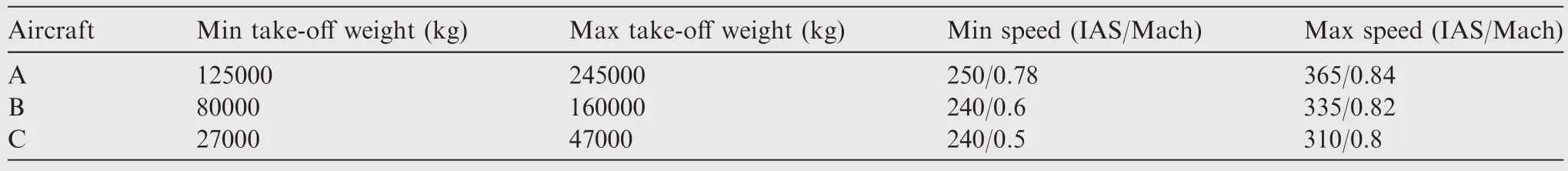
Table 2 Aircraft general characteristics.

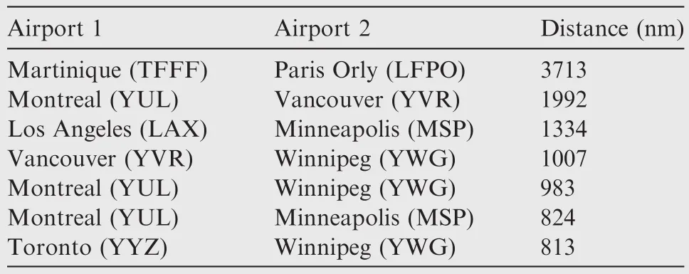
Table 3 Flight distances for different trajectories.

Table 4 shows the Flight Cost,the number of nodes(branches)pruned at Levels 1,2,and 3–4,the total number of nodes(Leaves)not evaluated as a consequence of the pruned branches,and the required computation time for seven differentCopt1values,and for aCopt2=0.65 for Aircraft A.

For aCopt1close to 0,a pessimist coefficient value,more branches are pruned at the highest level(Level 1),thus reducing the algorithm execution time.This fact can be seen forCopt1＜0.6.However,this fast computation brings with it the consequence that the global optimal cost was not found,because the branch that contained the optimal solution was pruned at a higher level due to theCopt1pessimism value.According to the results in Table 3,for aCopt1＞=0.6,the optimal trajectory was always found;however,the computation time was considerable higher.For these same tests,for aCopt1＜0.6,the algorithm was not able to find the optimal result.However,for a different flight,the solution might be found for aCopt1＜0.6.

The computation time is directly related to the number of leaves evaluated,as illustrated in Table 3,where for aCopt1=0,a total of 9270 possible trajectories(leaves)were not evaluated(more branches were pruned)using the real cost,which lead to a computation time of 8.1 s.A total of 5610 possible trajectories were not evaluated (less branches were pruned)with aCopt1=0.8,which lead to a computation time of 280.2 s.Obviously,Copt1needs to be adjusted to the required value in order to obtain very good results.

Copt2also has an important effect on the pruning process,as seen in Table 5,where the same flight as the one shown in Table 4 was executed,but with a less optimisticCopt2=0.2.

It is clear that the ‘Flight Cost” value is the same in Tables 4 and 5,which shows the importance ofCopt1in finding the optimal solution.Copt2contributes to rejecting the last node to be evaluated by increasing the number of leaves not evaluated.For aCopt1＞0.6,the computation time was reduced for around 100 s in the results in Table 4(Copt2=0.2)compared against the results in Table 3(Copt2=0.65).This computation timereduction isduetothenumberof branches/leaves not evaluated at the 3rd and 4th levels due to theCopt2pessimist in Table 4.

4.1.2.Optimism coefficient and its effects in convergence of algorithm

The developed algorithm tends to converge to the optimal solution as itwas seen in the results provided by Tables 4 and 5.However,the convergence was affected by the selection of parametersCopt1andCopt2.

By selecting high values ofCopt,the algorithm converges to the optimal solution(12,587 kg)at the expenses offlight time.By selecting low values ofCopt,the algorithm also converges to the optimal solution,but fails to deliver the optimal solution staying in a ‘close” local optimal(12,616 kg).Selecting the right combination ofCoptvalues makes the algorithm to systematically converge to the optimal solution.

4.2.Beam Search Algorithm and Exahustive Search Algorithm

The BSA was compared with the ESA(which guarantees the global optimal)for different flights to measure the quality of the solution.For these sets of tests,the standard atmosphere was used,and the Cost Index=0,since the goal of these tests was to observe if the optimal flight profile was found.This test was performed for three different aircraft.

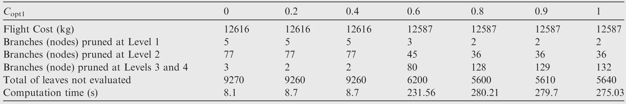
Table 4 Optimism coefficient results of Winnipeg to Montreal flight for Copt2=0.65.

4.2.1.Aircraft A

The airports considered in the tests were Montreal(YUL),Vancouver(YVR),Toronto(YYZ),Winnipeg(YWG),Minneapolis(MSP),Los Angeles(LAX),Martinique(TFFF)and Paris Orly(LFPO).For aircraft A,the number of possible leaves(flight combinations)is close to 15730.Table 6 shows the optimal cost for each of the flights by means of an Exhaustive Search Algorithm and by the Beam Search Algorithm developed in this paper.

For the evaluation of Aircraft A,the coefficients values wereCopt1=0.6 andCopt2=0.2.The flight cost was compared in Table 5 as calculated by the Exhaustive(first row)and the Beam Search(second row)algorithms.This comparison showed that 6 out of 7 flights provided the same cost,while for one trajectory,the flight cost difference was of only 44 kg.In order to find the optimal flight cost,theCopt1should be higher to make the evaluating function more ‘optimistic”,this way,fewer nodes(branches)would be pruned and the optimal flight might be found.However,incrementing theCopt1as seen in Tables 3 and 4 would increment the computation time.

As shown in Table 6,the algorithm was capable of not evaluating up to 9350 leaves due to pruned nodes(branches)for the flight YUL-YYZ in Table 6.This means that only around 30%of the space search was evaluated(4690 leaves).

4.2.2.Aircraft B

For this Aircraft,the total number of leaves(flight combinations)is around 4320.As with Aircraft A,Table 7 shows the optimal flight cost trajectories found by using the ESA versus the trajectories found with the developed BSA.

The algorithm was able to find the optimal solution for all flight cases.The optimism coefficients used for aircraft B were:Copt1=0.6 andCopt2=0.1.The numbers of nodes(branches)note evaluated are shown in Table 7.Cases such as the Los Angles(LAX–Minneapolis(MSP)can be found,where the search spacewasexplored onlyby28% (1070leaves evaluated).

4.2.3.Aircraft C

For this aircraft,the total number of leaves(flight combinations)is close to 6468.As with Aircraft A,and Aircraft B,Table 8 gives the results found for Aircraft C.In the same way,the ESA flight is compared against the developed BSA.Since this is a medium-range aircraft,the destinations considered are different from the destinations for the other aircraft(Aamp;B).The new airport added is Chicago(ORD).

For Aircraft C,the algorithm is able to find the optimal trajectory for all flights.For these tests,the optimism coefficients areCopt1=0.6 andCopt2=0.1.The number of nodes(branches)and leaves(flight combinations)not evaluated is shown in Table 8.For this aircraft,it can be seen that for the YYZ-ORD flight,only around the 10%(624 flight combinations)of the search space was evaluated.

4.3.BSA and results obtained from FMS/PTT

It will be useful to determine if the BSA is able to improve the trajectories suggested by the FMS/PTT.A flight cost comparison between the optimal trajectories generated by the FMS/PTT and the optimal trajectory generated by the algorithm developed in this paper was executed.The FMS/PTT is consid-ered as a black box since the methodology used in the FMS/PTT is confidential.

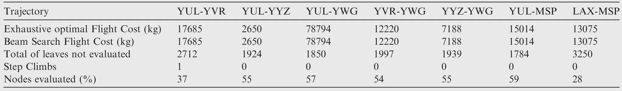
Table 7 Algorithm performance for Aircraft B.

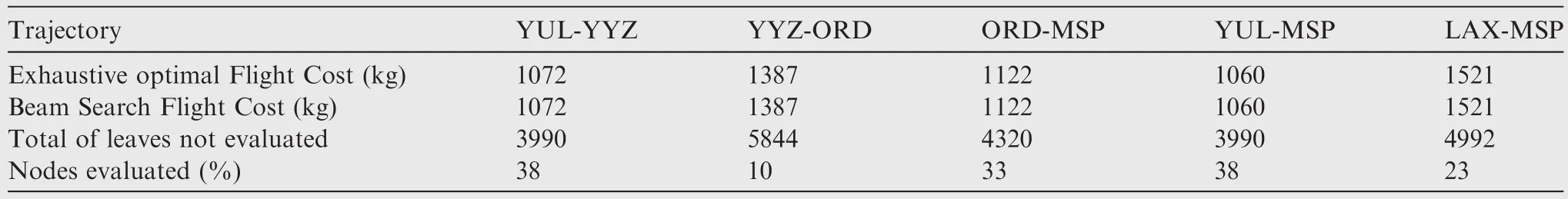
Table 8 Algorithm performance for Aircraft C.

To make this comparison,inputs were introduced first in the FMS/PTT,obtaining the optimal VerticalFMS/PTTreference profile.The same inputs were then introduced to the BSA to obtain the optimal VerticaALGOreference profile.The costs of both Vertical reference profiles were calculated using the ‘real cost computation” method(see tion 2.2),and these costs were compared to observe the flight cost differences between the commercial FMS and the developed algorithm.

The ‘input parameters” were:the initial and final destination points,the reference Lateral Navigation trajectory,the Cost Index and the initial aircraft weight.

For Aircraft B,a flight from Montreal to Vancouver was simulated varying the Cost Index up to 90.The results are visualized in Fig.5,and show the variation of the flight cost with the Cost Index.

As illustrated in Fig.5,the algorithm developed in this paper reduced the flight cost with the generated vertical reference trajectories than with the reference FMS/PTT.

4.4.BSA considering wind influence

Weather information was obtained from the Environment Canada website.The parameters of interest were the wind speed,the wind direction,the temperature and the pressure.The tests performed in this section validated if the developed algorithm was able to find the optimal(or near-optimal)solution by considering the stochastic wind influence.

Firstly,an Exhaustive Search was performed for different flights by considering the available weather information.The same flights were executed using the algorithm developed in this paper.The flight costs obtained using both algorithms(BS and ES)were compared and the results difference between both algorithms is shown in Fig.6.

As expected,when the weather influence was introduced,the algorithm was not always able to converge to the optimal solution,and for the flights tests set,only two flights,as shown in Fig.6(Flight 1 and Flight 2)provided the optimal solution.This lack of convergence was obtained because the heuristics fail to capture the wind influence;thus,nodes corresponding to the optimal solution were pruned.Very good suboptimal solutions were found because the ‘worst” solution(Flight 4 in Fig.6)was only 0.34%more expensive than the optimal solution.

The optimal solutions provided by the Exhaustive Search and by the BSA for Flight 2 in Fig.6 are shown in Table 8.The developed algorithm was executed for that flight with the same weather information for different values ofCopt1and an arbitrary constantCopt2=0.3.The initial gross weight was of 120000 kg.Results are found in Table 9.

Table 9 Optimal flight provided by ESA.

Table 10 Results provided by ‘Beam Search” algorithm considering weather.

The results in Table 10 show that,as expected,the number of pruned branches decreases as the coefficient is less optimistic.

5.Conclusion

This paper described an algorithm to optimize the vertical reference flight trajectory by using a numerical performance model.The problem was solved using a decision tree in the implementation of the deterministic ‘Beam Search” algorithm.The ‘Optimism Coefficient” has influenced the algorithm’s aggressiveness.The algorithm made a compromise between flight time and fuel burn optimization.Fuel burn reduction has a direct effect in the reduction of polluting emissions,which are known to cause global warming and health problems.Therefore,the developed algorithm,taking advantage of ‘step climbs” and ‘weather parameters” to calculate the optimal aircraft trajectory,was conceived by taking into account ATM constraints such as constant Mach and constant altitude segments following a pre-defined lateral reference route.

The algorithm’s ability to reduce the number of possible combinations by up to 86%in some cases,was clearly demonstrated.This brings us a consequence of a low computation time,which is desirable for low computation power avionics devices such as the FMS.It was also shown that by correctly selecting the ‘optimism coefficients”,the algorithm found the optimal solution in many different flight cases.

It has been observed that the solutions found by the algorithm for different cost indexes were always more economical than the results obtained using a commercial FMS.

As future work,it is desirable to improve the heuristics when implementing the weather.It will be worthwhile to analyze the flights of a larger number of aircraft operating in the same airspace to obtain the algorithm’s performance in the presence of other aircraft or even other constraints such as Non-Fly Zones.It would also be of interest to develop a new technique to determine the best locations to realize step climbs instead of using constant trajectories at fixed time or fixed distance points.

Acknowledgements

We would like to thank the team of the Business-led Network of Centers of Excellence Green Aviation Researchamp;Development Network(GARDN),and in particular Mr.Sylvan Cofsky,for the funds received for this project(GARDN II–Project:CMC-21).This research was conducted at The Research Laboratory in Active Controls, Avionics and Aeroservoelasticity(LARCASE)in the framework of the global project ‘Optimized Descent and Cruise”.For more information please visit http://larcase.etsmtl.ca.We would like to thank Mr.Rex Haygate,Mr.Dominique Labour,Mr.Oussama Abdul-Baki,Mr.Reza Neshat and Mr.Yvan Blondeau from CMC-Electronics–Esterline,and Mr.Oscar Carranza from LARCASE for their invaluable contributions.We also would like to thank CONACYT and FQRNT.

1.International Air Trasnport Association.Vision 2050.Geneva;Switzerland:IATA;2011.

2.Gill M.Aviation:benefits beyond borders.Geneva,Switzerland:Air Transport Action Group(ATAG);2014.

3.International Civil Aviation Organization.Aviation’s contribution to climatechange,ICAO environmentalreport.Montreal,Canada:International Civil Aviation Organization(ICAO);2010.

4.Freitag W,Shulze ET.Blended winglets improve performance.Aeromag Boeing2009;35:9–12.

5.International Air Trasnport Association.Beginner’s guide to aviation biofuels.Geneva,Switzerland:IATA;2009.

6.McConnachie D,Wollersheim C,Hansman JR.The impact offuel price on airline fuel efficiency and operations.Proceedings of 2013 aviation technology,integration,and operations conference,Aug 12–14;Los Angeles(CA),USA.Reston(VA):AIAA;2013.

7.Randt NP,Jessberger C,Ploetner KO.Estimating the fuel saving potential of commercial aircraft in future fleet-development scenarios.Proceedings of the 15th AIAA aviation technology,integration,and operations conference;2015 June 22–26;Dallas(TX),USA.Reston(VA):AIAA;2015.

8.Cao Y,Kotegawa T,Sun DF,DeLaurentis D,Post J.Evaluation of continuous descent approach as a standard terminal airspace operation.Proceedings of the 9th USA/Europe air traffic management research and development seminar;2011 June 14–17;Berlin,Germany.2011.

9.Clarke JP,Brooks J,Nagle G,Scacchioli A,White W,Liu SR.Optimized profile descent arrivals at Los Angeles international airport.J Aircraft2013;50(2):360–9.

10.Kwok-On T,Anthony W,John B.Continuous descent approach procedure development for noise abatement tests at louisville international airport,KY.AIAA’s 3rd annual aviation technology,integration,and operations(ATIO)forum;2003 November 17–19;Denver(CO),USA;Reston(VA):AIAA;2003.

11.Tong KO,Boyle DA,Warren AW.Development of continuous descent arrival(CDA)procedures for dual-runway operations at houston intercontinental.Proceedings of the 6th AIAA aviation technology,integration and operations conference(ATIO);Sep 25–27.Wichita(Kansas),USA.Reston(VA):AIAA;2006.

12.Murrieta-Mendoza A,Botez RM,Ford S.Estimation of fuel consumption and polluting emissions generated during the missed approach procedure.Proceedings of the 33nd IASTED international conference on modelling,identification,and control(MIC 2014);2014 Feb 17–18;Innsbruck,Austria.Calgary:IASTED;2014.

13.Dancila R,Botez RM,Ford S.Fuel burn and emissions evaluation for a missed approach procedure performed by a B737-400.Reston(VA):AIAA;2014.Report No.:AIAA-2014-4387.

14.Nangia R.Operations and aircraft design towards greener civil aviation using air-to-air refuelling.AeronautJ2006;110(1113):705–21.

15.Godbole PJ,Ranade AG,Pant RS.Branchamp;bound global-search algorithm for aircraft ground movement optimization.Proceedings of the 14th AIAA aviation technology,integration,and operations conference;2014 June 16–20;Atlanta(GA),USA.Reston(VA):AIAA;2014.

16.Jensen LL,Hansman RJ,Venuti J,Reynolds TG.Commercial airline altitude optimization strategies for reduced cruise fuel consumption.Proceedings of the 14th AIAA aviation technology,integration,and operations conference;2014 June 16–20;Atlanta(GA),USA.Reston(VA):AIAA;2014.

17.Jensen L,Hansman RJ,Venuti JC,Reynolds T.Commercial airline speed optimization strategies for reduced cruise fuel consumption.Proceedings of 2013 aviation technology,integration,and operations conference;2013 Aug 12–14;Los Angeles(CA),USA.Reston(VA):AIAA;2013.

18.Filippone A.On the benefits of lower Mach number aircraft cruise.Aeronaut J2007;111(1122):531–42.

19.Bonnefoy PA,Hansman RJ.Operational implications of cruise speed reductions for next generation fuel efficient subsonic aircraft.Proceedings of the 27th congress of the international council of the aeronautical sciences;2010 Sep 19–24;Nice,France.Bonn:ICAS;2010.

20.Turgut ET,Cavcar M,Usanmaz O,Canarslanlar AO,Dogeroglu K,Armutlu K,et al.Fuel flow analysis for the cruise phase of commercial aircraft on domestic routes.Aerosp Sci Technol2014;37:1–9.

21.Valenzuela A,Rivas D.Optimization of aircraft cruise procedures using discrete trajectory patterns.J Aircraft2014;51(5):1632–40.

22.Franco A,Rivas D.Minimum-cost cruise at constant altitude of commercial aircraft including wind effects.J Guidance Contr Dynam2011;34(4):1253–60.

23.Pargett DM,Ardema MD.Flight path optimization at constant altitude.J Guidance Contr Dynam2007;30(4):1197–201.

24.Franco A,Rivas D.Optimization of multiphase aircraft trajectories using hybrid optimal control.J Guidance Contr Dynam2015;38(3):452–67.

25.Houacine M,Khardi S.Gauss pseudospectral method for less noise and fuel consumption of aircraft operations.J Aircraft2010;47(6):2152–8.

26.McEnteggart Q,Whidborne J.A multiobjective trajectory optimisation method for planning environmentally efficient trajectories.2012UKACCinternationalconferenceoncontrol(CONTROL);2012 Sep 3–5;Cardiff,UK.Piscataway(NJ):IEEE Press;2012.p.128–35.

27.Guo X,Zhu M.Direct trajectory optimization based on a mapped Chebyshev pseudospectral method.Chin J Aeronaut2013;26(2):401–12.

28.Miyazawa Y,Wickramasinghe NK,Harada A,Miyamoto Y.Dynamic programming application to airliner four dimensional optimal flight trajectory.Proceedings of AIAA guidance,navigation,and control(GNC)conference;2013 Aug 19–22;Boston(MA),USA.Reston(VA):AIAA;2013.

29.Ng HK,Sridhar B,Grabbe S.Optimizing aircraft trajectories with multiple cruise altitudes in the presence of winds.J Aerosp Inform Syst2014;11(1):35–47.

30.Hagelauer P,Mora-Camino F.A soft dynamic programming approach for on-line aircraft 4D-trajectory optimization.Eur J Oper Res1998;107(1):87–95.

31.Cobano JA,Alejo D,Heredia G,Ollero A.4D trajectory planning in ATM with an anytime stochastic approach.Proceedings of the 3rd international conference on application and theory of automation in command and control systems;2013 May 28–30;Naples,Italy.New York:ACM;2013.

32.Rippel E,Bar-Gill A,Shimkin N.Fast graph-search algorithms for general-aviation flight trajectory generation.J Guidance Contr Dynam2005;28(4):801–11.

33.Wang HL,Lyu WT,Yao P,Liang X,Liu C.Three-dimensional path planning for unmanned aerial vehicle based on interfered fluid dynamical system.Chin J Aeronaut2015;28(1):229–39.

34.Chen YB,Yu JQ,Mei YS,Zhang SY,Ai XL,Jia ZY.Trajectory optimization of multiple quad-rotor UAVs in collaborative assembling task.Chin J Aeronaut2016;29(1):184–201.

35.Dancila BD,Botez RM,Labour D.Fuel burn prediction algorithm for cruise,constant speed and level flight segments.Aeronat J New Ser2013;117(1191):491–504.

36.Dancila BD,Botez RM,Labour D.Altitude optimization algorithm for cruise,constant speed and level flight segments.Proceedings of AIAA guidance,navigation,and control conference;2012 Aug 13–16;Minneapolis(Minnesota),USA.Reston(VA):AIAA;2012.

37.Fe´lix-Patro´n RS,Kessaci A,Botez RM.Horizontal flight trajectories optimisation for commercial aircraft through a flight management system.Aeronaut J New Ser2014;118(1210):20.

38.Murrieta-Mendoza A,Botez RM.Lateral navigation optimization considering winds and temperatures for fixed altitude cruise using the Dijkstra’s algorithm.Proceedings of ASME international mechanical engineering congressamp;exposition;2014 Nov 14–20;Montreal,Canada.New York:ASME;2014.

39.Collinson RPG.Introduction to avionics systems.3rd ed.Dordrecht(Netherlands):Springer Science+Business Media B.V;2011.

40.Gagne´J,Murrieta-Mendoza A,Botez R.New method for aircraft fuel saving using flight management system and its validation on the L-1011 aircraft.Proceedings of 2013 aviation technology,integration,and operations conference;2013 Aug 12–14;Los Angeles(CA),USA.Reston(VA):AIAA;2013.

41.Murrieta-Mendoza A,Botez RM.Vertical navigation trajectory optimization algorithm for a commercial aircraft.Proceedings of AIAA/3AF aircraft noise and emissions reduction symposium;2014 June 16–20;Atlanta(GA),USA.Reston(VA):AIAA;2014.

42.Felix Patron RS,Botez RM,Labour D.New altitude optimisation algorithm for the flight management system CMA-9000 improvement on the A310 and L-1011 aircraft.Aeronaut J New Ser2013;117(1194):787–805.

43.Murrieta-Mendoza A.Vertical and lateral flight optimization algorithm and missed approach cost calculation[dissertation].Montre´al:E´cole de Technologie Supe´rieure;2013.

44.Fe´lix-Patro´n RS,Oyono-Owono AC,Botez RM,Labour D.Speed and altitude optimization on the FMS CMA-9000 for the Sukhoi Superjet 100 using genetic algorithms.Proceedings of 2013 aviation technology,integration,and operations conference;2013 Aug 12–14;Los Angeles(CA),USA.Reston(VA):AIAA;2013.45.Fe´lix-Patro´n RS,Berrou Y,Botez RM.New methods of optimization of the flight profiles for performance databasemodeled aircraft.Proc Inst Mech Eng Part G J Aerosp Eng2015;229(10):545–57.

46.Fe´lix-Patro´n RS,Botez RM.Flight trajectory optimization through genetic algorithms coupling vertical and lateral profiles.Proceedings of ASME 2014 international mechanical engineering congressamp;exposition;2014 Nov 14–20;Montreal,Canada.New York:ASME;2014.

47.Murrieta Mendoza A,Demange S,George F,Botez RM.Performance database creation using a level D simulator for cessna citation X aircraft in cruise regime.Proceedings of the 34th IASTED International conference on modelling,identification,and control(MIC2015);2015 Feb 16–18;Innsbruck,Austria.Calgary,Canada:IASTED;2015.

48.Murrieta-Mendoza A,Botez RM.Methodology for verticalnavigation flight-trajectory cost calculation using a performance database.J Aerosp Inform Syst2015;12(8):519–32.

49.Sabuncuoglu I,Bayiz M.Job shop scheduling with beam search.Eur J Oper Res1999;118(2):390–412.

50.Ojha SK.Optimization of cruising flights of turbojet aircraft.Flight Performance of Aircraft.Reston(VA):AIAA;1995.p.237–58.

19 August 2016;revised 22 September 2016;accepted 28 October 2016

Available online 21 June 2017

*Corresponding author.

E-mail address:ruxandra.botex@etsmtl.ca(R.M.BOTEZ).

Peer review under responsibility of Editorial Committee of CJA.

Production and hosting by Elsevier

http://dx.doi.org/10.1016/j.cja.2017.06.006

1000-9361©2017 Chinese Society of Aeronautics and Astronautics.Production and hosting by Elsevier Ltd.

This is an open access article under the CC BY-NC-ND license(http://creativecommons.org/licenses/by-nc-nd/4.0/).

Beam search;

Commercial aircraft;

Flight time;

Flight management system;

Fuel burn;

FMS;

Trajectory optimization