Wenquan Zhou(周文权),Jincheng Wang(王锦程),†,Zhijun Wang(王志军),Yunhao Huang(黄赟浩), Can Guo(郭灿),Junjie Li(李俊杰),and Yaolin Guo(郭耀麟)

1 State Key Laboratory of Solidification Processing,Northwestern Polytechnical University,Xi’an 710072,China

2 Ningbo Institute of Industrial Technology,Ningbo 315201,China

Elastic strain response in the modified phase-field-crystal model∗

Wenquan Zhou(周文权)1,Jincheng Wang(王锦程)1,†,Zhijun Wang(王志军)1,Yunhao Huang(黄赟浩)1, Can Guo(郭灿)1,Junjie Li(李俊杰)1,and Yaolin Guo(郭耀麟)2

1 State Key Laboratory of Solidification Processing,Northwestern Polytechnical University,Xi’an 710072,China

2 Ningbo Institute of Industrial Technology,Ningbo 315201,China

To understand and develop new nanostructure materials with specific mechanical properties,a good knowledge of the elastic strain response is mandatory.Here we investigate the linear elasticity response in the modified phase-field-crystal (MPFC)model.The results show that two different propagation modes control the elastic interaction length and time,which determine whether the density waves can propagate or not.By quantitatively calculating the strain field,we find that the strain distribution is indeed extremely uniform in case of elasticity.Further,we present a detailed theoretical analysis for the orientation dependence and temperature dependence of shear modulus.The simulation results show that the shear modulus reveals strong anisotropy and the one-mode analysis provides a good guideline for determining elastic shear constants until the system temperature falls below a certain value.

elastic response,strain distribution,shear modulus,modified phase-field-crystal model

1.Introduction

The elasticity of materials is important for understanding processes ranging from the propagation of elastic waves,to flexure,and to brittle failure.[1–4]A complete parameterization of elastic properties in experiments is however challenging,especially for the deformation of a solid which operates across several length and time scales.Usually,the elastic deformation dynamics on atomic length(∼10−10m)and time (∼10−12s)scales can be captured by molecular dynamics (MD)simulations.[5]However,due to very short time scales, only high stresses(GPa)and strain rates(107s−1)can be probed in the dynamical deformation process.These are to be contrasted with much slower experimental strain rates of 10−5 s−1 to 10−3 s−1.[6]

Recently,based on the density functional theory,[7]Elder and Grant[8,9]proposed a new methodology,called the phasefield crystal(PFC)model,which provides a natural description of slow,diffusive dynamics in interacting systems while still maintaining the atomic-level resolution,including topological defects,elasticity,and plasticity.This method has powerful capabilities in describing polycrystalline solidification,[10,11]phase transitions,[12]vacancy diffusion dynamics,[13]dislocation(annihilation,glides and climb),[14,15]and fracture.[16,17]As to the elasticity and plasticity behaviors,[18,19]the PFC method can also describe mechanical responses at low stress and low steady-state strain rate.Considering that the original PFC model did not contain a mechanism for describing elastic interactions sufficiently,Stefanovic et al.[18,20,21]proposed a modified phase-field-crystal(MPFC)model in which the corresponding dynamic equation includes the inertia effect or wave-like term∂2ϕ/∂t2originated from the second order term of time.Thus this MPFC can facilitate rapid elastic relaxations.After comparing results from MPFC to those from PFC,Stefanovic et al.found that the elastic relaxation presented in the MPFC is consistent with the linear elasticity theory.However,the details of a parameter interval for the elasticity behavior are still lacking and how the crystal lattice orientation or system temperature influences the elastic coefficients is also unclear.Therefore,in this work,we first investigate the elastodynamic response of the MPFC model by analyzing the deformation behavior of a strained nano-single crystal specimen,and then we quantitatively characterize the strain distribution of the specimen and analyze the effects of the initial crystal lattice orientation and temperature on the shear modulus.One of the primary goals of this work is to gain new physical insight into these problems,which will prompt the MPFC method as a predictive tool to capture the elastic response of atomic properties for more complicated real materials.

2.Model description and strain characterization

2.1.The MPFC model

The PFC model was introduced to describe periodic systems of a continuum field and can naturally incorporate elastic and plastic behaviors.It relies on a well-known Swift–Hohenberg(SH)form free energy functional and an over damped equation of motion in describing the temporal evolution of the field ϕ that represents the reduced local particle density.The simplest dimensionless PFC model for pure systems follows as a conserved evolution of the free energy

where the order parameter ϕ is the atom number density field measured from a constant reference value,and r is a phenomenological constant related to the temperature.

The standard dimension less evolution kinetic equation for the order parameter ϕ is

The above kinetic equation describes time scales in crystals near and beyond that of the characteristic vacancy diffusion time.It does not,however,allow any collective atomic oscillations,which are on a much faster time scale.This omission of elastic interactions in the model prevents us from studying phenomena involving several time scales of various orders of magnitude(such as the deformation dynamics of nanocrystalline solids).To tackle this problem,the MPFC dynamic equation is introduced by adding a second order time derivative to the equation[18]

where α and β are phenomenological constants related to the effective sound speed and vacancy diffusion coefficient,respectively.Equation(3)is of the form of a damped wave equation,and it supports two density propagating solutions: one diffusional and the other corresponding to a propagation elastic mode.By choosing effective values of α and β,finite elastic interaction length and time can be set.

The thermodynamic properties of the PFC model have been discussed previously,[8,9,22]indicating that this model can yield different crystal phases,such as body-centered-crystal lattices,hexagonal lattices,and lamellar phase.The periodic order parameter ϕ can be written in the general form

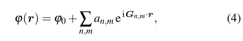
where an,mis the amplitude of the atomic density,r is the space position vector,and ϕ0is the average atomic density. Gn,m≡n b1+m b2,where b1and b2are the reciprocal lattice vectors.For two-dimensional(2D)hexagonal lattices,these reciprocal lattice vectors can be written as

where a0is the crystal lattice constant.Here we employ onemode approximation to keep the only critical mode whose amplitude is equal to A/4(A is the amplitude of the density waves).The hexagonal lattice density in two dimensions is acquired as

where q is the wave number related to a0,satisfying q= 2π/a0.Substituting Eq.(6)into Eq.(1),integrating over a unit cell,and minimizing the free energy with respect to A and q lead to

The physical details of all parameters and the solving procedure of Eq.(3)spectrally implemented in the Fourier space can be referenced to Ref.[23].Here,unless otherwise specified,all parameters used in the simulation are

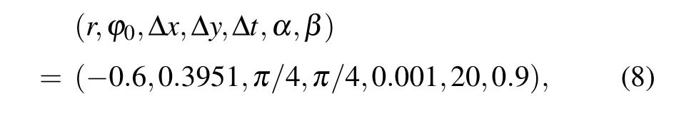
where Δx and Δy are the grid-sizes and Δt is the time-step size.

2.2.The elastodynamic response in the MPFC model

If we consider a perfect lattice with one“atom”chopped out,this would correspond to a vacancy in the lattice.Phonon vibrations would occasionally cause neighboring atoms to jump into the vacancy and eventually the vacancy would diffuse through the lattice.In the PFC model,the density at the vacancy slowly fills in and the density at the neighboring sites slowly decreases as the vacancy diffuses throughout the lattice. To determine time scales of vacancy diffusion,it is useful to perform a linear stability analysis,[24]which linearizes Eq.(2) around an equilibrium state density field ϕeqaccording to

where Q is a perturbation wave vector and bn,m(t)is the corresponding amplitude associated with the perturbation of the steady-state mode(n,m).The resulting linearized equation of Eq.(2)is obtained by substituting Eqs.(9)–(11)into Eq.(2) and expanding the latter to linear order.Then the diffusion constant can be obtained as

This analysis demonstrates that equation(2)admits propagating solutions for density disturbances with an effective diffusion time tD,which can be written as

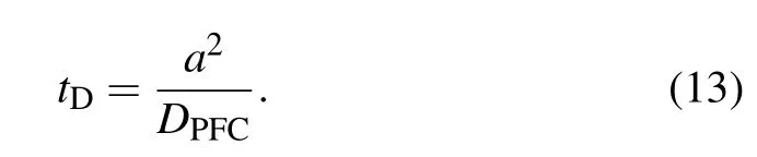
Take Cu at 1063°C as an example.With a lattice parameter of a=3.61˚A and the self-diffusivity D≈10−13m2·s−1, it will take about tD=1.30µs for an atom to diffuse to its original nearest neighbor position.On the other hand, the bond stretch“vibrational period”[25]is estimated to be tv≈2π(ma2/EB)1/2≈1 ps,where m≈64 u is the atom mass and EB≈1 eV is the binding energy due to the interatomic potential.So tD≫tv,note that the diffusive motion of an atom in the crystalline phase is much larger than the elastodynamic response time of the vibrational motion of an atom.This suggests that elastic strains will relax instantly,implying that the system would correspond to an over-damped system,which prevents PFC simulation from direct comparison with faster, real-world mechanical experiments.In order to overcome this deficiency,the MPFC model was introduced to make the PFC model operating on two time scales:one diffusional and the other corresponding to a propagating elastic mode.[18]

To better understand the diffusive dynamics and elastic interactions governed by the MPFC equation,a linear stability analysis is performed.The linearized equations are the same as Eqs.(9)–(11).It is straightforward to repeat the above calculation in the PFC model.Substitute Eqs.(9)–(11)into Eq.(3)and ignore higher-order nonlocal terms retaining only the contribution b0,0among the nonlinear coupling terms with zero modes.By solving the resulting linearized dynamic equation,the effective elastic interaction length and interaction time can be obtained(see Ref.[18]for details)

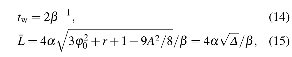
By properly tuning the parameters α and β,finite elastic interaction length and time can be set.Over this elastic interaction time and distance,the density waves will propagate effectively undamped.Beyond this time and distance,however, the density evolution becomes diffusive.As an illustration, considering a system with dimension L,we require the elastic interaction lengthwhich impliesAfter choosing an appropriate value for α,β can be determined from β=α2Δ/DMPFC.Using Cu at 1063°C as an example(D≈10−13m2·s−1)and the computational domain L=1µm,one would choose the effective sound speedα=3.16×10−7m/s and the effective vacancy diffusion coefficient β=0.16 s−1.If we compare this sound speed with that in the classical MD simulations(α∼103m/s),we can obtain αMD/αMPFC∼1010,implying that MD is 1010times faster.

In short,the MPFC approach takes advantage of the fact that elastic relaxation does not need to be instantaneous due to a separation of elastic relaxation and diffusion time scales.

3.Results and discussion

In this section,several simulation results are shown to demonstrate the abilities of MPFC formulation in describing the elasticity response at atomistic scales.Firstly,we will discuss the shear deformation response of the MPFC model,and then examine the elastic response of a nano-single crystal.Finally,the orientation and temperature dependence of the shear modulus will also be discussed.

All the simulations performed in this part are conducted in a rectangle domain of size 1024Δx×1024Δy,i.e.,a 1024× 1024 grid.A nano-single crystal sample with hexagonal lattices(two-dimensional)is placed in the domain L×H= 77a0×109a0=[150Δx,874Δx]×[Δy,1024Δy].A small coexisting liquid boundary of width 150Δx is included on both left and right sides of the sample.The reason why we use coexisting liquid at the boundaries is the requirement of solving the dynamics equation in the MPFC model efficiently.Usually,the dynamics equation is spectrally implemented in the Fourier space,thus the boundary conditions should be periodic in all directions.So,to satisfy this requirement,the free surfaces are created by choosing chemical potential to vary spatially over narrow strips near the solid–liquid interfaces of the system.This is accomplished by choosing values of r and ϕ0from the coexistence region of the hexagonal solid and liquid phase diagram.[8,9]By using a lever rule,the amounts of liquid and solid in the simulated sample are set with no preference toward crystallization or melting,i.e.,a stable interface arises at the boundary.Thus the sample could be considered as having periodic boundary conditions at y=1 and y=1024 and free boundary conditions elsewhere.Several of the following simulations require the incorporation of external loads.After the sample has equilibrated(the relaxed state in Fig.1(a)),the atoms within the narrow strips(white line with an arrow in Fig.1(b))at x1=150 and x1=874 are dragged at a constant velocity v=10−4along the y-axis in opposite directions(the relaxed state in Fig.1(b)).This is accomplished by adding an external function to the original free energy functional[26]

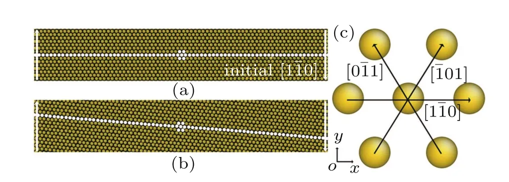
Fig.1.(color online)(a)Atom density field of a nano-single crystal specimen in a relaxed state and(b)in a strained state during shear deformation.Note that only a portion of the simulation sample is shown here. (c)The white atoms in panel(a)are enlarged,which can schematically illustrate the(111)plane in a hexagonal close-packed crystal lattice in two-dimensions.

3.1.Shear deformation response

To demonstrate the presence of elastic relaxation modes in the MPFC model,we performed simulations of a nanosingle crystal specimen as described above(the initial crystal orientation equals to zero)under shear deformation.In the PFC paradigm,the crystal atoms can be interpreted as the discrete set of maxima of the continuous density field.Figure 2(a) shows the position in the case of the row of atoms in[1¯10] direction(depicted by white atoms in Fig.1(a))at four different strain levels.Here,the atom position was extracted by using the atomic position detection(APD)method,[27]where the locations of local maxima in the atom density field were tabulated after each time-step.When the dragged atoms are displaced by an amount D0,which is vertical to the initialdirection,a linear displacement distribution,D(y)= D0(y)/(µL)(µis the shear modulus),will be established.The data(Fig.2(a)with β=0.9)clearly show that the crystal response is consistent with elasticity theories,as shown by the rigid tilting of atoms in thedirection.At the same time, we can conclude that equation(3)can describe the elastic response in strained crystals at finite strain rates.

On the other side,for β=20,the crystal atoms fail to react fast enough to the shear deformation and the behavior is viscoelastic,as shown in Fig.2(b).What is more,the curve fails to obey a linear displacement distribution.It means that the shear strain wave can only propagate with a limited range. In Fig.2(c),the propagating range W of the strain wave is plotted with respect to the parameter β.When 0＜β＜1, the propagating range stays constant(shown in the insert of Fig.2(c)),which indicates that in this parameter range,the system reveals an elastic response.When β＞1,the curve decreases dramatically.In this case,the system corresponds to very over damped dynamics and could model the viscoelastic behavior.With the above analysis,we know that if we want to simulate the elasticity response of the system,we should choose the parameter β in elasticity regimes(0＜β＜1).

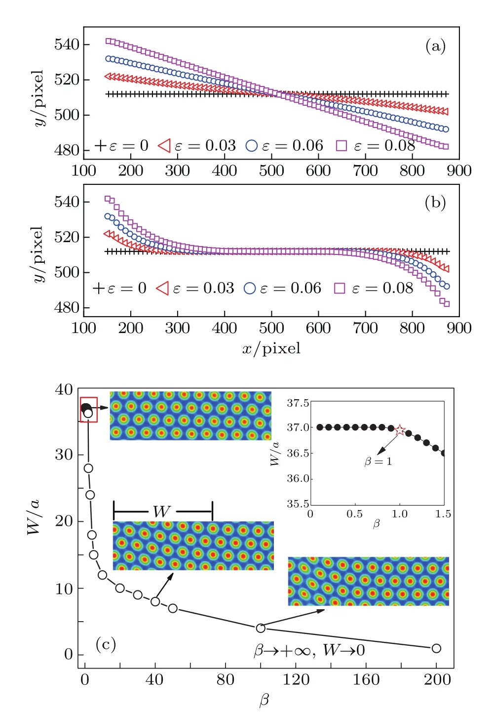
Fig.2.(coloronline)Precisely detectatomic position along the row of atoms in[1¯10]direction of the nano-single crystal at four strain levels with different effective vacancy diffusion coefficients:(a)β=0.9,(b)β=20.(c)The propagating range W of the strain wave is plotted with respect to the parameter β.The inset shows the enlarged images of the region enclosed in the red shadow box.

3.2.Strain distribution in shear deformation

The purpose of this section is to demonstrate that the MPFC approach can be used to investigate the elastic strain response at atomic scales.In continuum models of a 2D lattice,distortions of the lattice can be defined by numerical differentiation[28]

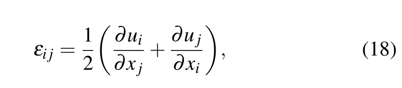
where εijdescribes the total strain tensor.The strains εxxand εyyrepresent the isotropic dilation(or compression)components,while εxyis the shear component(anti-clockwise positive).In order to obtain these strain components,here we use a numerical image-processing technique named as the peak pairs analysis(PPA)to precisely determine the strain field at atomic length scales.The details of the method can be referenced to Refs.[28]and[29].

We have characterized the strain distribution forthe specimen(the initial crystal orientation equals to zero)described in Fig.2(a)in Subsection 3.1.Figure 3 shows the shear strain (εxy)distribution contours during shear deformation at four different strain levels.Figures 3(a)–3(c)reveal a gradual increase in the shear strain from the dragged atoms to the core of the specimen during deformation.This is evidenced by the gradual change in color from orange to green and to light blue. Finally,there is an almost homogeneous distribution within the whole specimen(Fig.3(c)),which will be confirmed in the following parts.Figure 3(d)shows the strain response to external applied strains.During the whole deformation process, the values of εxxand εyycan be considered to be almost zero, and εxyis a linear function of the applied strain.According to the linear elastic theory,the theoretical value of the applied shear strain(engineering)is twice of shear strain εxy.The corresponding simulated result is εxy=0.5807εappliedstrain,indicating the quantitative consistency with the elastic theory.

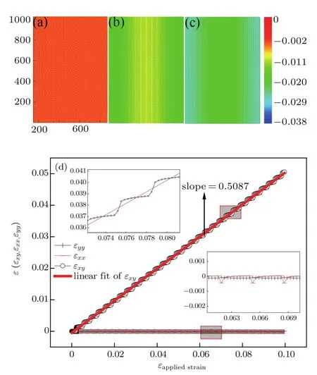
Fig.3.(color online)Shear strain field maps of εxy calculated over the nanosingle crystal specimen(Fig.1(a))at three different strain levels respectively: (a)εapplied=0,(b)εapplied=0.0347,(c)εapplied=0.0679.The color bar represents the variation of the shear strain,the positive value means counterclockwise rotation of the lattice and the negative value represents the opposite rotation.(d)The curves of shear strain ε(εxx,εyy,εxy)response to the external applied strain(εappliedstrain),ε is obtained by averaging the strains of all the atoms across the sample.The inset shows the enlarged images of the region enclosed in the red shadow box.

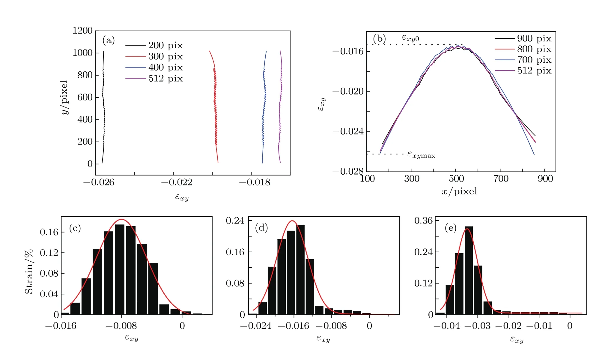
Fig.4.(color online)Shear strain distributions over the nano-single crystal specimen.Strain data in panels(a)and(b)are extracted from the four fixed line regions in Fig.3(c)at different coordinate values(pixels).Strain data in panels(c)–(e)are acquired through counting the strains of all the atoms in Figs.3(a)–3(c),respectively,and the red solid line is the Gaussian profile.

To illustrate the strain distributions in the local areas, the strain pattern is further examined.Figure 4(a)shows the variation of the strain extracted from the line regions,parallel to the applied shear direction at four fixed x pixels in Fig.3(c).The shear patterns in Fig.4(a)are approximately linear,which means that the strain wave propagates with the same velocity along the x direction.In contrast,figure 4(b) shows the same variation of strain but the line regions vertical to the applied shear direction at four fixed y pixels in Fig.3(c). We can note that all the curves(Fig.4(b))are close to a symmetric distribution with the minimum strain value at the center and with the maximum value near the dragged atoms,with Kt=εxy(max)/εxy(0)=1.795(Ktis defined as the strain concentration),the value is in excellent agreement with the previous analysis results,[30]in which the value is 1.8.To illustrate the strain distributions in the whole area of the specimen,the shear strain evolving distribution histograms are further examined(Figs.4(c)–4(e)).These histograms are gained through counting the strains of all the atoms in the specimen (Fig.3(c)).From Figs.4(c)–4(e),we can see that the Gaussian profile matches the strain distribution extremely well without regard to those atoms with a strain value very near zero.Furthermore,the widths of the strain distributions are almost the same.Thus we can confirm that the strain distribution in the specimen interior is extremely uniform during the whole stage of deformation.

3.3.Orientation dependence of the shear modulus

The magnitude of the material’s elastic anisotropy plays an important role in elastic interactions.Here we show how anisotropy enters into the model.The shear modulus of the hexagonal crystal can be obtained by calculating the energy costs for deforming the equilibrium state.First,we can consider perturbations of the density field in an equilibrium state (Eq.(6)),i.e.,

In such calculation,ξ represents the dimensionless strain.According to Wu’s work,[31]for small strains,we can set the q value equal to the wave number of the unstrained state,and assume the amplitude A is the same for simplicity.To determine the elastic energy,we substitute Eq.(19)into the free energy functional of Eq.(1),which can be explicitly evaluated in terms of A,q,and ξ.Then minimizing the resulting free energy with respect to ξ yields

where α=(qA)2.To the lowest order in ξ,the elastic energy density can be expressed as

The elastic constants are then C44=α/4 and the shear modulusµ=C44.But the above analytical calculation has not considered the orientation dependence of the shear modulus.Characterizing the modulus of the hexagonal crystal needs two variants,the shear constant C44and an orientation factor,as a function of θ,where the angle is defined between thecrystal direction and the directions of x-axis(perpendicular to the loading direction).For the purpose of coupling the density field and the crystal orientation,we need to start the calculation from the model.First choose two basic reciprocal lattice vectors(b1and b2)with the magnitude described in Eq.(5),and a coordinate rotation maps the two variables into new variablesso as to determine the directions.The coordinate rotation can be described as(j= 1,2).Then the density field containing crystal orientation can be obtained asTo obtain the elastic energy density,we substitute ϕ′(r)into the free energy functional(Eq.(1))and again use the same procedure described in Eqs.(1),(9),and(11).

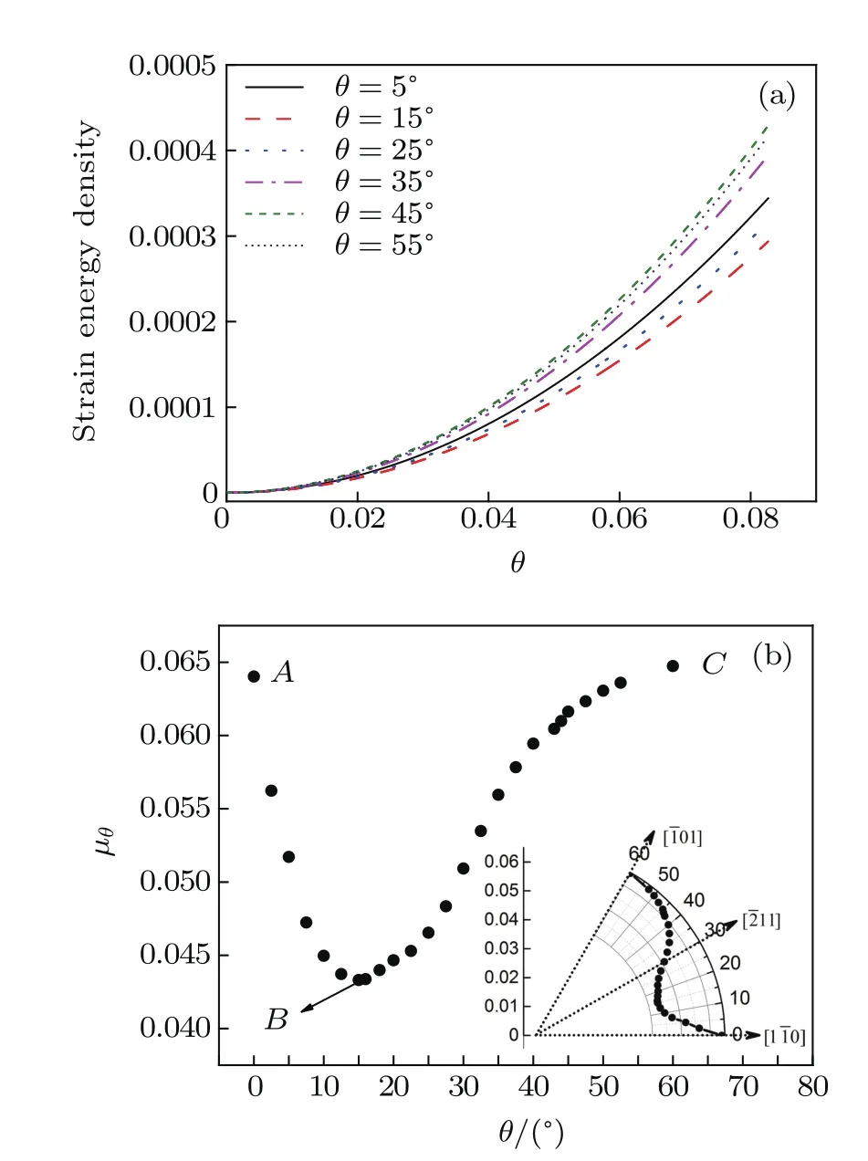
Fig.5.(color online)(a)Elastic strain energy density calculated from the MPFC simulations with different initial orientations of hexagonal lattice.(b)Orientation dependence of shear modulus µθ.The inset shows the polar plot ofµθ.

We have given a general analysis procedure for calculating the orientation dependence of the shear modulus.Since the analytical calculation is too cumbersome when adding the crystal direction angle θ to the free energy functional,here we focus only on the numerical approach to investigate how the angle θ influences the shear modulus.To accomplish this,we repeat the similar simulation in Subsection 3.2 with the same domain size and the same related parameters.The only difference is that the nano-single crystal specimens are sheared with different initial crystal orientations.Figure 5(a)shows the calculated elastic energy with different orientation angles. The energy change trends are consistent in all situations and strictly fitted to the quadratic form of Eq.(21),where the shear constant C44is easily extracted.Figure 5(b)shows the orientation dependence of shear modulus(µθ).Due to the symmetry of the hexagonal structure,when the angle θ equals to zero or 60°,µθreaches the maximum at the same time shown as points A and C in Fig.5(b),which correspond to the[1¯10]and [¯101]directions,respectively(shown in the inset).However, when the shear direction in not parallel to the main crystal direction,at the angle θ of about 15°,µθreaches the minimum (point B in Fig.5(b)).Traversing from the whole curve,we can find that the shear modulus reflects the high anisotropy.

3.4.Temperature dependence of the shear modulus

In this part,we show the dependencies between the temperature r and the shear modulus µr.The effective temperature r modulates the magnitude of the amplitude of the hexagonal crystal,which changes the shear modulus.In Subsection 3.3, we have obtained the relationship µr=α/4=(qA)2/4,where

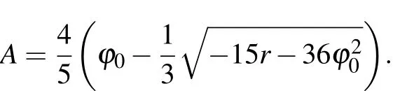
Thus the analytic solutions can be easily obtained.What is more,for the numerical solutions,we also repeat the similar simulation in Subsection 3.2 with the same domain size and the related parameters.The only difference is that the specimens are sheared with different initial temperatures.Figure 6 shows the calculated elastic energy with different temperatures.The energy change is also fitted to the quadratic form of Eq.(21).The upper left inset of Fig.6(a)shows the enlarged images of the region enclosed in the red shadow box,which shows that although the differences between these curves are very close to each other,it can make a big difference in the magnitude of the shear modulus.Figure 6(b)compares the analytic and numerical solutions of shear modulusµrfor a variety of values of r.The results show that the numerical solutions ofµrdecrease linearly with increasing temperature (red solid line).For the analytic solutions,it is quite close to the numerical solutions and becomes exact when the absolute value of r is small enough,but a deviation from the numerical solutions occurs when the system temperature falls below a certain value at r=−0.665.This deviation can be attributed to the hexagonal lattice contraction due to the nonlinear coupling of the principle reciprocal lattice vectors to higher order reciprocal lattice vectors.[31]Thus the analytic results can in principle be systematically improved by including higher orders in the expansion of the density field.

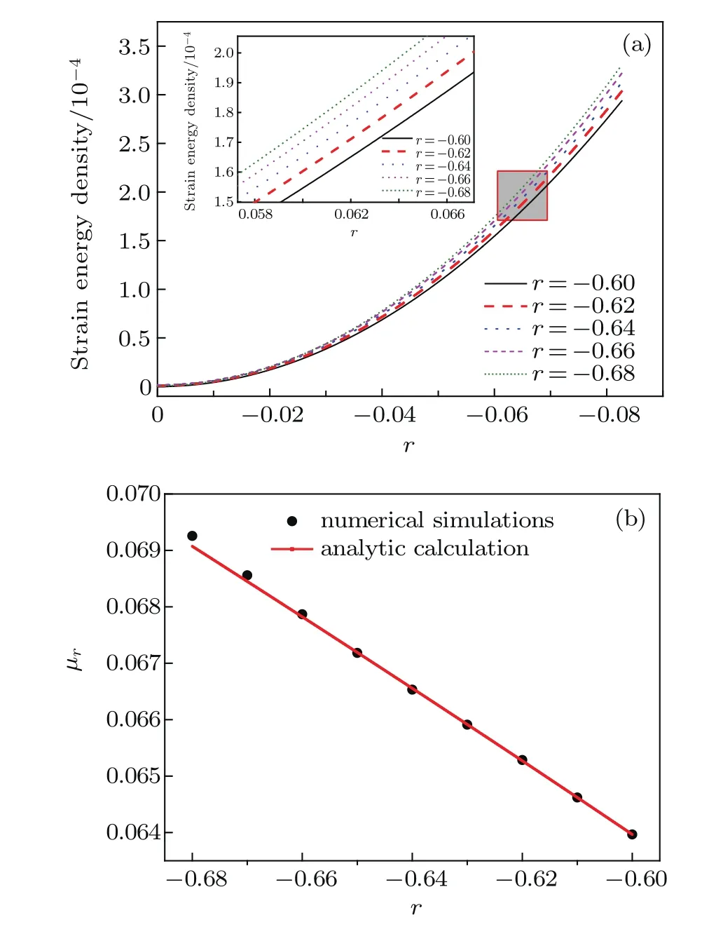
Fig.6.(color online)(a)Elastic strain energy density calculated from the MPFC simulations as a function of temperature r.The inset shows the enlarged images of the region enclosed in the red shadow box.(b) Temperature dependence of shear modulusµr.The red solid line is an analytic calculation and the black points are from numerical simulations.

4.Conclusion

We have presented the elastic properties of hexagonal crystal in the context of the MPFC model.This methodology allows propagating sound modes as long as 0＜β＜1.Values of 1＜β would correspond to over damped dynamics and reveal viscoelastic behavior.We have also quantitatively characterized the strain distribution of the specimen.The results show that when statisticed along the shear direction the strain pattern reveals approximately linear,when statisticed vertical to the shear direction,it is close to a symmetric distribution.

We have also presented a detailed theory analysis for determining elastic shear constants when they depend on the various parameters in the free energy functional of hexagonal crystal.The one-mode analysis provides a good guideline for determining coefficients of nonlinearities of elastic energy to obtain the shear constants.The shear constantµθreveals strong anisotropy;this phenomenon is intrinsically related to the nonlinear coupling of the principle reciprocal lattice vectors to the crystal orientation.In the case of temperature dependence of the shear modulus,our analytical results obtained in the one-mode approximation are borne out qualitatively by numerical simulations until the system temperature falls below a certain value.

A highly interesting perspective is the extension of this work to use multi-mode calculations for a more accurate evaluation of the shear constants.The calculation of the constants performed here remains valid when considering the amplitude and lattice constant changed with temperature due to the higher-order reciprocal lattice vectors.What is more,a huge volume fraction of defects,such as surfaces and grain boundaries,exist in the nanostructured crystals.Linea and nonlinear elasticity constitute important contributions to the latter plastic deformation of the nanostructures.Further study of this phenomenon by using the MPFC model would be of great interest.

Acknowledgment

We thank the Center for High Performance Computing of Northwestern Polytechnical University,China for computer time and facilities.

[1]Zhu T and Li J 2010 Prog.Mater.Sci.55 710

[2]Du J P,Wang Y J,Lo Y C,Wan L and Ogata S 2016 Phys.Rev.B 94 104110

[3]Chen L Y,Richter G,Sullivan J P and Gianola D S 2012 Phys.Rev. Lett.109 125503

[4]Wang Y J,Gao G J and Ogata S 2013 Appl.Phys.Lett.102 041902

[5]Dao M,Lu L,Asaro R J,Hosson D J and Ma E 2007 Acta.Mater.55 4041

[6]Hessam Y and Kianoosh H 2015 Model.Simul.Mater.Sci.23 065004

[7]Oxtoby D W 2002 Ann.Rev.Mater.Res.32 39

[8]Elder K R and Grant M 2004 Phys.Rew.E 70 051605

[9]Elder K R,Katakowski M,Haataja M and Grant M 2002 Phys.Rew. Lett.88 245701

[10]Wu K A and Karma A 2007 Phys.Rev.B 76 184107

[11]Yang T,Chen Z,Zhang J,Wang Y X and Lu Y L 2016 Chin.Phys.B 26 057802

[12]Guo C,Wang J C,Wang Z J,Guo Y L and Tang S 2015 Phys.Rev.E 92 013309

[13]Chan P Y,Goldenfeld N and Dantzig J 2009 Phys.Rev.E 79 035701

[14]Ren X,Wang J C,Yang Y J and Yang G C 2010 Acta Phys.Sin 59 3595 (in Chinese)

[15]Gao Y J,Huang L L,Deng Q Q,Zhou W Q,Luo Z R and L K 2016 Acta.Mater 117 238

[16]Gao Y J,Luo Z R,Huang L L,Mao H,Huang C G and Lin K 2016 Model.Simul.Mater.Sci.24 055010

[17]Hu S,Chen Z,Peng Y Y,Liu Y J and Guo L Y 2016 Comp.Mater.Sci. 121 143

[18]Stefanovic P,Haataja M and Provatas N 2006 Phys.Rev.Lett.96 225504

[19]Zhou W Q,Wang J C,Wang Z J,Zhang Q,Guo C,Li J J and G Y L 2017 Comp.Mater.Sci.127 121

[20]Stefanovic P,Haataja M and Provatas 2009 Phys.Rev.E 80 046107

[21]Chan P Y,Tsekenis G,Dantzig J,Dahmen K A and Goldenfeld N 2010 Phys.Rev.Lett.105 015502

[22]Wu K A and Voorhees 2012 Acta.Mater 60 407

[23]Adland A,Karma A,Spatschek R,Buta D and Asta M 2013 Phys.Rev. B 87 024110

[24]Provatas N and Elder K R 2011 Phase-field Methods in Materials Science and Engineering(Urbana:Wiley)p.158

[25]Wang Y Z and Li J 2010 Acta Mater.58 1212

[26]Trautt Z T,Adland A,Karma A and Mishin Y 2012 Acta Mater 6528

[27]Wang Z J,Guo Y L,Tang S,Li J J,Wang J C and Zhou Y H 2015 Ultramicroscopy 150 74

[28]Calindo P L,Kret S,Sanchez A M,Laval J Y,Yanez A,Pizarro J, Guerrero E,Ben T and Molina S I 2007 Ultramicroscopy 107 1186

[29]Hytch M J,Snoeck E and kiaas R 1998 Ultramicroscopy 74 131

[30]Pilkey W D and Pilkey D F 2008 Peterson’s Stress Concentration Factors(New York:Wiley)p.105

[31]Wu K A and Voorhees 2009 Phys.Rev.B 80 125408

21 February 2017;revised manuscript

6 May 2017;published online 18 July 2017)

10.1088/1674-1056/26/9/090702

∗Project supported by the National Natural Science foundation of China(Grant Nos.51571165 and 51371151),Special Program for Applied Research on Super Computation of the NSFC-Guangdong Joint Fund(the second phase),China,and the Fundamental Research Funds for the Central Universities,China(Grant No.3102015BJ(II)ZS001).

†Corresponding author.E-mail:jchwang@nwpu.edu.cn

©2017 Chinese Physical Society and IOP Publishing Ltd http://iopscience.iop.org/cpb http://cpb.iphy.ac.cn