ZHOU Xue-ying, SUN Lin, WEI Jing, JIA Shang-feng, TIAN Xin-peng, WU Tong

Geomatics College, Shandong University of Science and Technology, Qingdao 266590, China

Analysis of Thermal Field Distribution in Winter over Beijing from1985 to 2015 Using Landsat Thermal Data

ZHOU Xue-ying, SUN Lin*, WEI Jing, JIA Shang-feng, TIAN Xin-peng, WU Tong

Geomatics College, Shandong University of Science and Technology, Qingdao 266590, China

Heat supply, automobile exhaust, industrial production and decrease of thermal inertia in winter caused by the decrease of vegetation coverage leads to an obvious difference in the distribution of the land thermal field in the winter compared with other seasons. The Urban thermal field distribution in the winter directly affects the spread of air pollutants, which has important implications for analyzing the contribution of the thermal field to particulate air pollution. Atmospheric transmissivity and atmospheric upwelling/downwelling radiance in simulations are first calculated using the moderate spectral resolution atmospheric transmittance algorithm and computer model (MODTRAN). Then, we solve the radiative transfer model of the thermal infrared band by constructing a look-up table. In addition, the accuracy estimation is performed using the simulated data, showing that when the error range of emissivity and water vapor content are confined to ±0.005 and ±0.6, respectively, the temperature retrieval error are less than 0.348 and 2.117 K, respectively indicating the high retrieval accuracy of the method. In addition, the long-term sequenced Landsat TM and ETM+ data were selected to retrieve land surface temperature (LST) during 1985-2015. The analysis of the temporal and spatial distribution of thermal fields in Beijing show that the spatial and temporal variations are observable. The spatial variation covers four levels: high temperature is distributed within the second ring, low temperature loops are distributed between the second and the fifth ring, high temperature is distributed in the outer suburb areas and the lowest temperature is distributed in the western mountainous areas. Meanwhile, the temporal variation of thermal field distribution changed a great deal during the rapid development in the past 3 decades: the low temperature loop expanded from the third to the sixth ring; the intensity and scope of the heat island effect within the second ring increased gradually.

Beijing; Winter; Thermal field distribution; LST; Landsat

Introduction

The acceleration of urbanization in Beijing since the 1980s has greatly changed the city environment. This affects the urban thermal field distribution[1]and directly influences the spread of air pollutants. The temperature in Beijing’s surrounding regions in the winter is lower compared with the temperature in the summer, which is influenced by the heat supply and exhaust gas emissions, etc. High temperatures appear in central Beijing in the winter, leading to a lower atmospheric pressure and impeding the diffusion of pollutants[2]. Meanwhile, coal burning causes the volume of pollutants to float to the central city as village residents warms themselves in the winter. Therefore, the study of the thermal field distribution and its variation in Beijing in the winter has great significance for understanding of the contribution of urban heat island to air pollution.

Remote sensing techniques play a crucial role in analyzing spatial temperature distributions. With the development of remote sensing technology, researches of urban thermal field distribution and variation have been widely performed using remote sensing techniques and multi-source remote sensing data. Gallo K P，et al. analyzed the thermal field distribution of 15 cities in Seattle using advanced very high resolution radiometer(VHRR) data of the NOAA satellite, which showed that the vegetation index has a strong relationship with the surface properties of suburb areas, and in the meantime, the urban heat island effect phenomenon has been evaluated using NDVI[3]; M. Stathopoulou et al. analyzed the urban heat island effect of coastal cities in Greece using AVHRR data from the NOAA satellite, which showed that port cities in Greece have obvious heat island effects caused by the dense population distribution, road network construction and frequent human activities[4]; Yang Yingbao et al. quantitatively analyzed the temporal and spatial characteristics of the heat island effect in Nanjing by combining Landsat TM data with MODIS data, which showed that the heat island effect is more apparent during the daytime and that the autumn the season has the strongest heat island effect while winter season has the weakest heat island effect[5]; U Rajasekar et al. monitored the strength of the heat island effect and spatial-temporal variation rules in Indianapolis by constructing a non-parametric model with TM and ETM+ data[6]; L Liu et al. performed a LST distribution retrieval in Hong Kong, indicating that the heat island effect primarily occurred in three suburb areas: Kowloon Island, northern Hong Kong Island and Hong Kong International Airport[7].

LST spatial distribution retrieval using remote sensing images in the thermal infrared band is a crucial method for analyzing the urban thermal field distribution. Presently, the complete algorithms of LST retrieval primarily include the single channel algorithm, multi-channel algorithm and multi-angle algorithm. The single channel algorithm refers to the acquisition of LST through radiant energy obtained by one thermal infrared channel on the satellite sensor, which is widely applied to the satellite sensor with only one thermal infrared band. With atmospheric vertical profile data (temperature, humidity and pressure profiles), this method can be used to determine the surface temperature through the use of an atmosphere transfer model. JC Price et al. firstly proposed a single channel formulation to standard meteorological soundings at a time near the overpass of an NOAA operational satellite, by which the retrieval accuracy of LST reached ±2～3 K[8]; Jiménez-Munoz presented an improved methodology to retrieve LST from AVHRR 4 and TM 6 using only water vapor as the input variable, and the results turned out that the mean RMSE was lower than 2 K for AVHRR channel 4 and 1.5 K for TM band 6[9]. A multi-channel algorithm is developed based on thermal data from several wavebands. Represented by the split-window algorithm, the algorithm was initially applied to AVHRR channels 4 and 5 to eliminate the atmospheric influence through radiant brightness differences of the two channels. First, Prabhakara proposed a split-window algorithm and applied it to the retrieval of sea surface temperatures[10]; later, this algorithm was amended and applied to the retrieval of LST; Rozenstein et al. applied the split-window algorithm to high-resolution Landsat 8 satellite[11]; Wan et al. modified the algorithm and applied it to the LST products of MODIS data[12]. A multi-angle algorithm means eliminating the atmospheric influence through various atmospheric paths under different observation angles. Chedin et al. simulated sea surface temperatures (SST) by a single-channel, double-viewing angle method using METEOSAT and TIROS-N and obtained a that the mean and the standard deviation between the retrieved and observed surface temperature of 0.2 and 1.2 K, respectively[13]; Sobrino et al. estimated the LST and SST using LOWTRAN-7 simulations from the Along-Track Scanning Radiometer (ATSR) data, and accuracies of approximately 1.5 K in LST are achievable[14]; He Liming et al. proposed that without atmospheric vertical profile data, the LST, which is retrieved by atmospheric-corrected AMTIS single-channel and multi-angle thermal infrared images, has a difference of 1K from the measured data[15].

This paper analyzes the thermal field distribution over Beijing in the winter using sequenced, long-term and high-resolution Landsat data. Landsat data over the most recent 30 years was retrieved. The LST was based on a different temporal scale based on the thermal infrared radiative transfer model. The thermal field distribution of Beijing was finally analyzed.

1 Data Sources

The landsat series is a land satellite program of NASA, collecting images from approximately 705 km above the surface in a sun-synchronous orbit with a 16-day revisiting period. The primary sensors include MSS, TM, ETM+ and OLI, which contain several discrete spectral channels, of which the spatial resolution of multi spectral channel is 30 m. The spatial resolutions for different thermal infrared channels are distinct, in which TM and ETM+ are 120 and 60 m respectively. So far, the Landsat series has been widely used in the retrieval of agriculture, forestry, natural disaster and environmental pollution monitoring[16-19].

In order to analyze the temporal and spatial variation rules of the thermal field distribution of Beijing in the winter from 1985 to 2015, this paper takes one Landsat image every five years as the research data. To guarantee its spatial integrity, images applied in this paper are of high quality. The cloud cover of the selected image is lower than 3% and Beijing is under free-cloud conditions. In addition, two of the high-quality images during December and the next January are selected to perform the experiment. Meanwhile, we try to maintain the same imaging time for the consistency of the phenological period over the 7 scenes from 1985 to 2015. Table 1 shows the specific data source information.

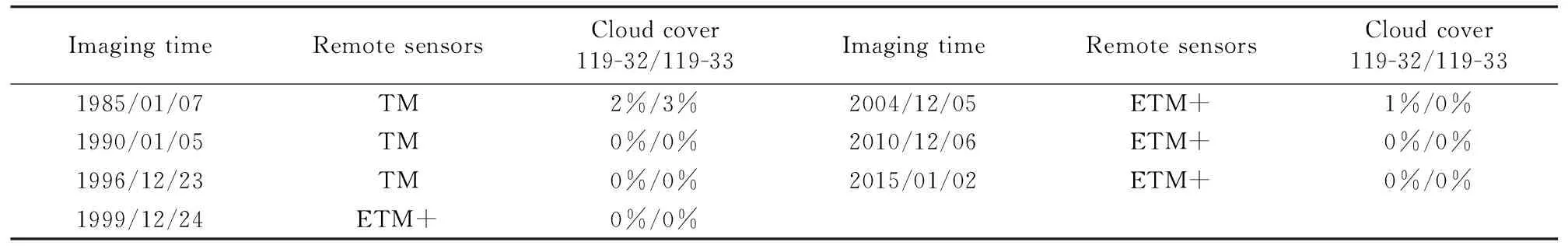
Table 1 Data source information

2 Surface Temperature Retrieval

2.1 Retrieval principle

The energy obtained by the thermal infrared radiation sensor includes three parts: the thermal radiance obtained by the sensor reflected by the land surface and then weakened by the atmosphere, the atmospheric downwelling radiance that is weakened again by the atmosphere after surface reflection, and the thermal radiance received by the sensor and atmospheric upwelling radiance. It can be derived from the equation

(1)

(2)

2.2 Determination of surface emissivity

The land surface can be simplified as a natural surface, urban area and water area, in which the natural surface is defined as composed of bare soil and vegetation. The emissivity of natural surface!pixelsεcan be calculated from the following equation[20]

ε=PvRvεv+(1-Pv)Rsεs+dε

(3)

whereεvandεsare the land surface emissivity (LSE) of vegetation and bare soil on the corresponding bands, respectively. For Landsat TM and ETM+,εv=0.986 07 andεs=0.972 15;RvandRsare the temperature retios of vegetation and bare soil, respectively, which are defined as follows

Rv=B6(Tv)/B6(Ts)

RS=B6(Tbs)/B6(Ts)

(4)

whereB6(Tv) andB6(Tbs) are the thermal radiant energy of vegetation and bare soil for the thermal infrared band, respectively;B6(Ts) is the radiant energy emitted by the land surface under the average surface temperatureTs. Similarly, urban areas can be defined as a mixture of urban and vegetation, thus, the LSE estimation equation is defined as follows

ε=PvRvεv+(1-Pv)Rmεm+dε

(5)

whereRmis the temperature ratio of construction. The temperature ratio of different land surface types can be calculated by the vegetation coverage as well

Rv=0.933 2+0.058 5Pv

(6)

Rs=0.990 2+0.106 8Pv

(7)

Rm=0.988 6+0.128 7Pv

(8)

(9)

wherePvis the vegetation coverage, which can be calculated by the Normalized Difference Vegetation Index (NDVI) . NDVIvand NDVISare NDVI of fully vegetation-covered pixels and bare soil pixels, valued at 0.7 and 0.05, respectively. Generally,dε=0 if the land surface is comparatively smooth; if the land surface has large altitude differences, the value ofdεcan be estimated according to the ratio of vegetation[21]. Water, whose emissivity is 0.995[22-23], is extracted through the modified normalized difference water index (MNDWI).

2.3 The determination of atmospheric transmittance and upwelling/downwelling

MODTRAN is adopted to simulate atmospheric upwelling/downwelling radiance and transmittance for the retrieval of LST. MODTRAN was developed jointly by the Air Force Research Laboratory/Space Vehicles Directorate and Spectral Sciences, Inc. using the FORTRAN language. It is mainly applied to accurately simulate of atmospheric transmittance and LST.

An atmospheric model and the water vapor content are needed in the simulation. MODTRAN 4 supplies several atmospheric models, in which the mid-latitude winter atmosphere is selected in this paper according to the condition of the research area and data source. The water vapor abundance is obtained from the parameter calculation tool for atmospheric correction that is published by NASA, and was proposed by Barsi in 2003. The Atmospheric Correction Parameter Calculator uses the National Centers for Environmental Prediction (NCEP) modeled atmospheric global profiles for a particular date, time and location as input[24]. Although the available data provided by NASA begins from 2000, the water vapor content that cannot be obtained is replaced by that of the same date from the previous year because the influence of water vapor in the whole research area is synthetic, and the water vapor content in the winter has small variations.

2.4 Accuracy validation

The data used in this paper are previous images, and there is no measurement that corresponds to them. Validation of the LST retrieval accuracy is performed by simulating the theoretical error of retrieved LST within the possible error range of each parameter via the radiative transfer model. LST retrieval is primarily affected by the surface emissivity and atmospheric water vapor content. With the aim of simulating error of retrieved LST using the above two parameters, atmospheric parameters are first simulated with the MODTRAN model, which is used to build the look-up table. Then the radiance value is obtained with the corresponding temperature, water vapor content and emissivity value. The retrieval of the corresponding LST can be conducted through the radiative transfer model in combination with the obtained radiance, water vapor content and emissivity data. The retrieved LST data are finally compared with the original standard data.

As major factors that affect retrieval accuracy, the influences of the emissivity and water vapor content on LST retrieval are analyzed separately. Taking emissivity as independent variable and confining it to an error range of ±0.005 with an interval of 0.001, the error range of LST is 0.068～0.348 K; taking the water vapor content as the independent variable and confining it to ±0.6 with an interval of 0.1, the LST error range is 0.318～2.117 K, indicating that the error range of the retrieved LST by the method is generally low.

3 Thermal field distribution analysis over Beijing in winter

Based on the above theories, this paper retrieves the winter LST from 1985 to 2015 in Beijing using Landsat TM/ETM+ data. Fig.1 is the spatial distribution of LST. The spatial distribution of the thermal field includes four parts: the western mountainous area, the suburbs, the area between the fifth and second ring and area within the second ring. The western, northwestern and northeastern parts of Beijing have lower temperatures because the vegetation coverage is relatively high. The suburb area has an overall higher land surface temperature, and an obvious annular belt of low temperature appears between the second and fifth ring. The LST of area within the central second ring is higher than that of the outer ring. Related studies prove that in an urban area, LST during the day is lower than in the suburb area in the winter, showing a distinct cold island effect[2]. In terms of time sequence, the LST of the western forest region increases during the early period of development. Owing to the measurements of returning farmland to forest and forest protection, the LST decreases gradually as the increase of forestland area yet when observing the overall variation, the annular belt of low temperature increases continuously with the expansion of the urban area.

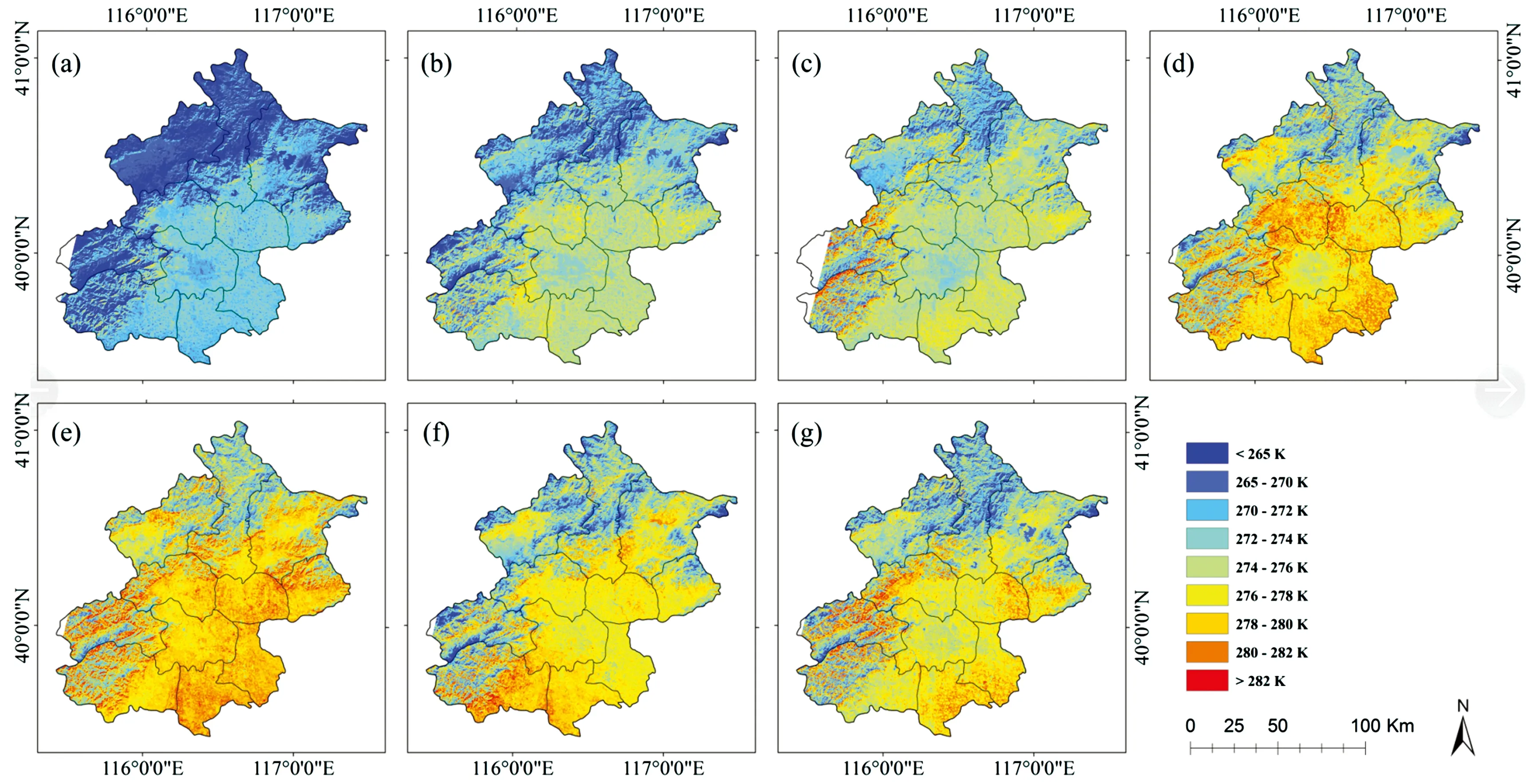
Fig.1 LST retrievals from 1985 to 2015 in Beijing

The mountainous area has the lowest LST in Beijing; in addition, the heat distribution differs remarkably as time changes. The mountains inside Beijing are approximately 2 000 m above sea level. As air temperature decreases with the increase of vertical height (the temperature drops approximately 0.6 ℃ for every 100 m increase in altitude), the surface temperature of the mountain area is the lowest. Moreover, the temperature between sunny slopes and shady slopes is distinct. Temperature differences in the mountainous area increased during 1985—2004, and large-scale low temperatures decreased gradually as the total temperatures increased; from 2010 to 2015, the low-temperature area expands due to the implementation of Beijing-Tianjin Sandstorm Source Control project. During this period, the forest coverage rate in Beijing increased by 5.7% according to figures released by the Landscaping department.

In order to analyze the temporal and spatial variation rules of the LST over central Beijing, the area between the ixth and the second ring is selected, as shown in Fig.2. Fig.3 shows the temperature distribution within the sixth ring, in which the blue outline marks the sixth and the second rings. The black area presents the region in which temperature is higher than average land temperature, while the white area presents the opposite. The red circle approximates the low temperature loop region, which gradually expands over the past 30 years, as is shown in Fig.3. Overall, the low temperature area is mainly distributed near the third ring in 1985 but expanded to the fifth ring in 2010 and the sixth ring in 2015 because of the accelerated urbanization process and continuous development of urban areas. Moreover, the low temperature area distributed radially in 2015, which was closely related to the construction of highway and railways and the surrounding economic development.

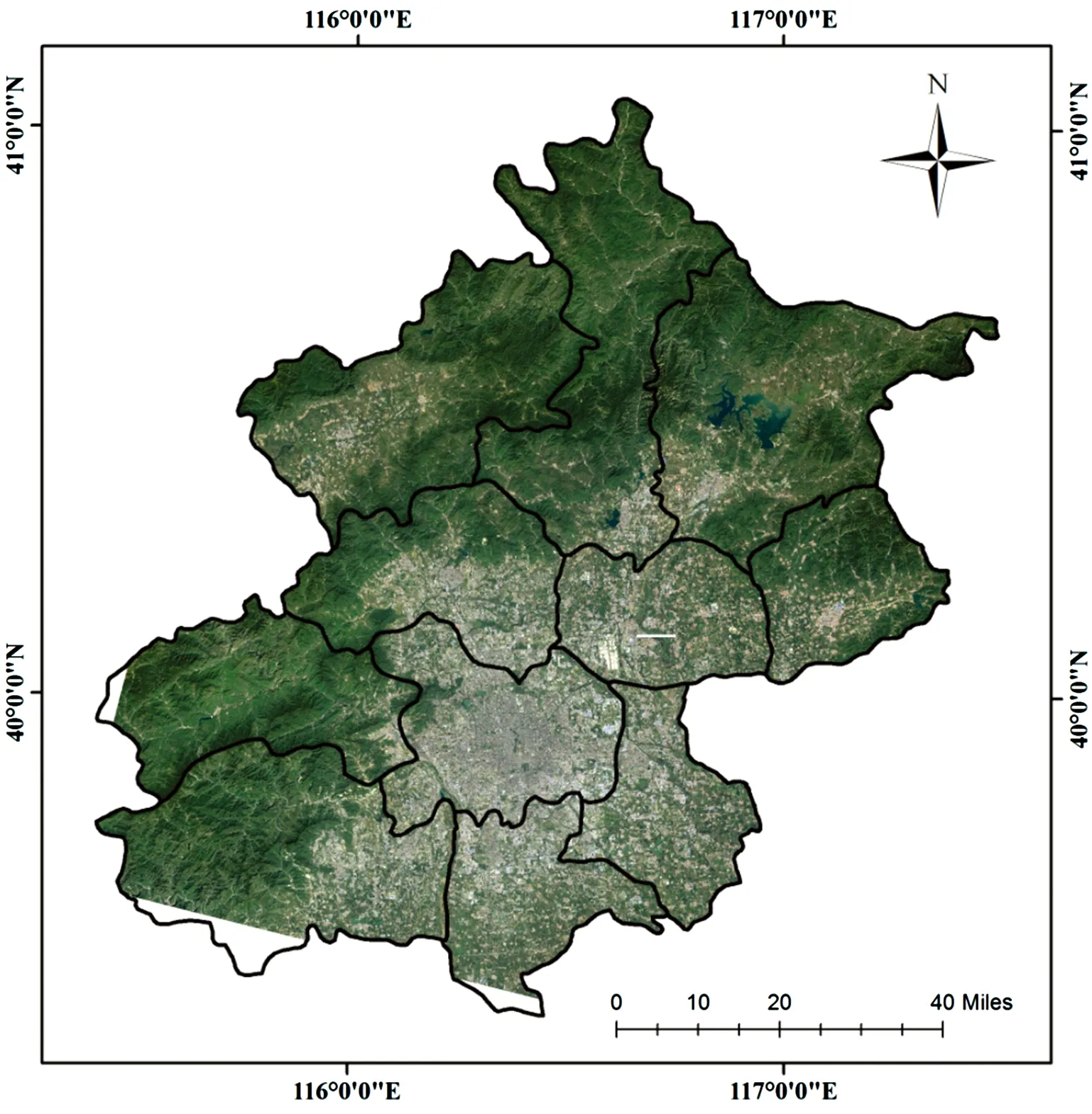
Fig.2 Scope of the study area

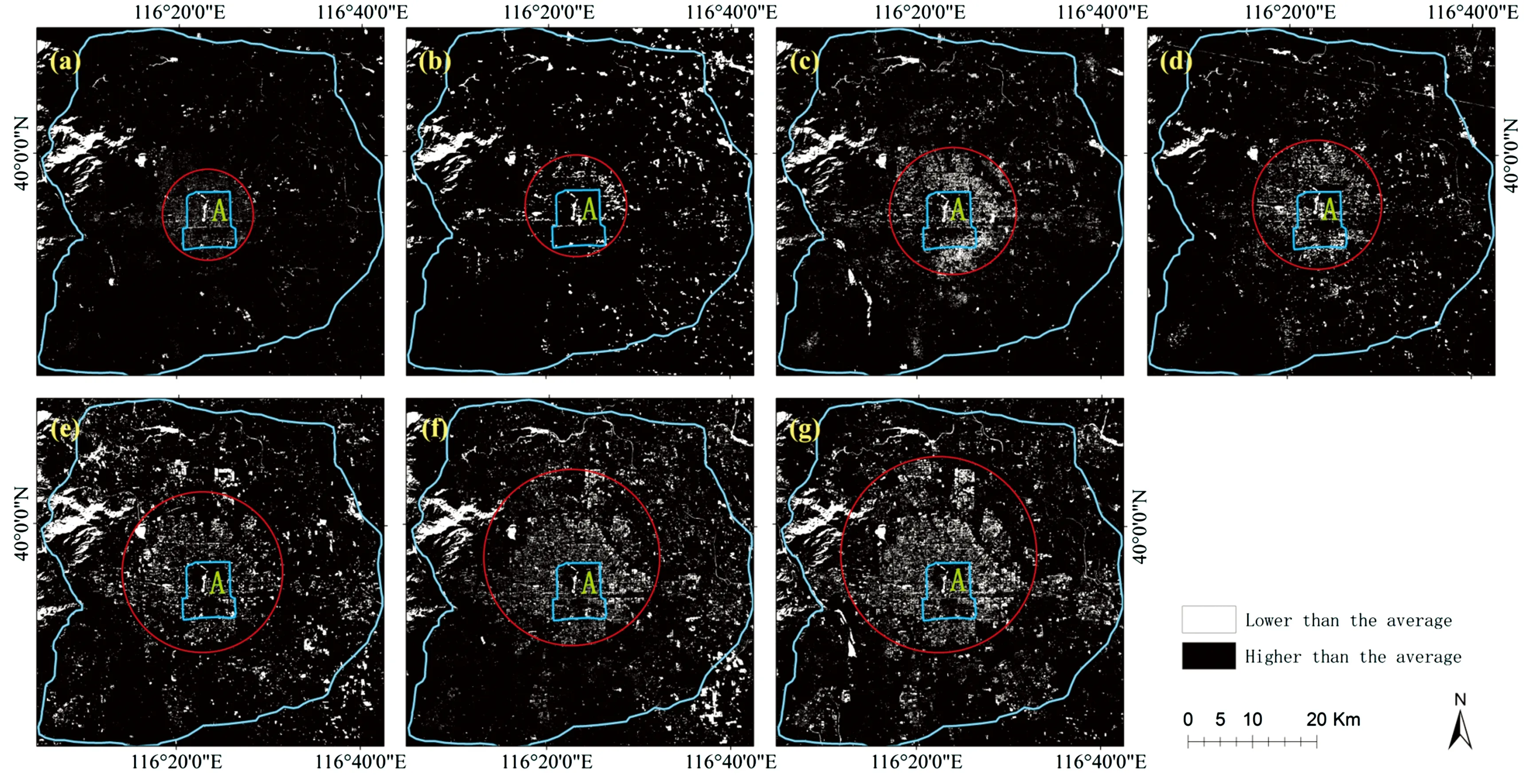
Fig.3 Distribution of low-LST urban areas in Beijing

The area within the second ring is the developed area with the most intensive population and the most frequent human activity. As shown in Fig.3, the overall LST is higher than that of surrounding areas, except for the water area A. With the aim of at analyzing the thermal field variation rule within the second ring, we performed a quantitative analysis on the LST variation with the Thermal Field Variance Index (TFVI)[25].

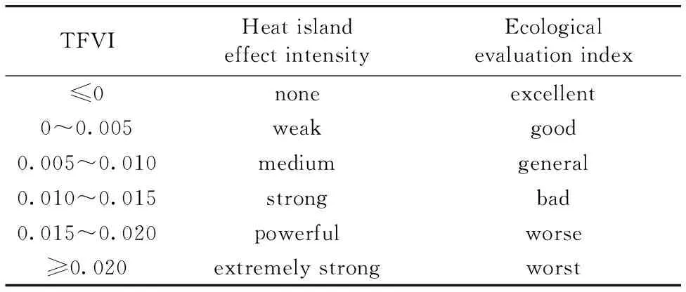
Table 2 Threshold division standard of the ecological evaluation index

TFVI=(T-TMEAN)/TMEAN

(10)

whereTis the LST of a specific point in the remote sensing image, andTMEANis the average LST value of the research area. As shown in Table 2, TFVI is classified into six grades in accordance with the ecological evaluation index.

Fig.4 shows the TFVI distribution within the second ring (the black outline) between 1985—2015, showing that the intensity of the heat island effect was lower before 1990; however, the weak heat island effect dominated until 2004 when a medium heat island effect appeared in the central region. Moreover, the medium and strong heat island effects emerged in 2010, and the total intensity continuously strengthened. A strong and powerful heat island effect continued in 2015, when an extremely strong heat island effect emerged. To give a more intuitive presentation of the variation trend of the heat island effect, Fig.5 gives the proportion of intensity within the second ring, in which none, weak and medium intensity is shown in the histogram since the proportion of other intensities is small. It is observed that the area with no heat island effect decreases gradually, from 91.80% to 41.81%; meanwhile, the area with a weak heat island effect increases from 8.05% to 33.96% and the area with medium heat island effect increases significantly, from 0.15% to 20.20%.

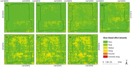
Fig.4 Distribution of urban heat island intensity in the second ring area of Beijing from 1985 to 2015

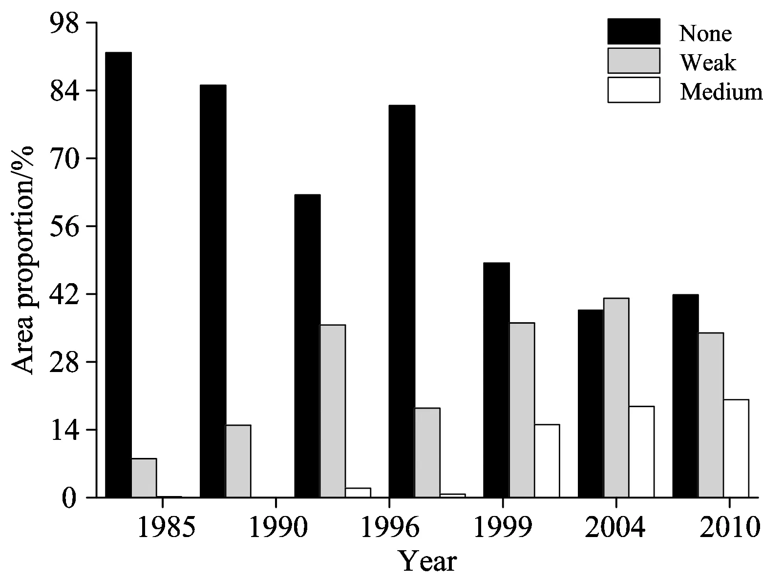
Fig.5 Area proportion of heat island effect intensity

4 Conclusion

This paper calculates three key atmospheric parameters using the MODTRAN atmospheric the radiative transfer model and solves radiative transfer equation of thermal infrared band by building a look-up table. The theoretical accuracy is evaluated through a simulation method, indicating the high retrieval accuracy and stability of the algorithm. We process Landsat TM/ETM+ data over the past 30 years for Beijing and perform LST retrieval based on a thermal infrared radiative transfer model. Then, we analyze the spatial distribution rule over Beijing in the winter, and the results show that the thermal field spatial distribution covers four parts: the area within the second ring has the highest temperature, resulting in the obvious heat island effect; the area between the fifth and second ring has an obvious low temperature loop; the temperature of the suburb area is high, and the temperature in the western mountainous area is the lowest. In addition, the temporal distribution rule indicates that the low temperature loop expands from the third to the sixth ring with the development of urbanization; in general, the intensity of the heat island effect within the second ring becomes stronger. Considering the long time span of the selected data and the difficulties in obtaining the measured LST data, this paper only evaluates the theoretical accuracy of the algorithm. Further research work will be focused on a more objective and reliable accuracy validation method.

[1] Wang Y, Xiao Y. Remote Sensing for Land & Resources, 2014, 26(3): 146.

[2] Wang J, Wang K, Wang P, Journal of Remote Sensing, 2007, 11(3): 330.

[3] Gallo K P, Mcnab A L, Karl T R, et al. Journal of Applied Meteorology, 2010, 325(5):899.

[4] Stathopoulou M, Cartalis C, Keramitsoglou I. International Journal of Remote Sensing, 2004, 25(12): 2301.

[5] Yang Y, Su W, Jiang N. Remote Sensing Technology & Application, 2006, 21(6): 488.

[6] Rajasekar U, Weng Q. International Journal of Remote Sensing, 2009, 30(30): 3531.

[7] Liu L, Zhang Y. Remote Sensing, 2011, 3(7): 1535.

[8] Price J C. Remote Sensing of Environment, 1983, 13(4): 353.

[10] Prabhakara C, Dalu G, Kunde V G. Journal of Geophysical Research, 1974, 79(33): 5039.

[11] Rozenstein O, Qin Z, Derimian Y, et al. Sensors, 2014, 14(4): 5768.

[12] Wan Z, Dozier J. IEEE Transactions on Geoscience & Remote Sensing, 1996, 34(4): 892.

[13] Chedin A, Scott N A, Berroir A. Journal of Applied Meteorology, 1982, 21(4): 613.

[14] Sobrino J A, Li Z L, Stoll M P, et al. International Journal of Remote Sensing, 1996, 17(11): 2089.

[15] He L, Yan G, Li X, et al. Journal of Infrared Millimeter Waves, 2006, 25(6): 429.

[16] Cristóbal J, Jiménez-Muoz J C, Sobrino J A, et al. Journal of Geophysical Research Atmospheres, 2009, 114(D8).

[17] Sun L, Wei J, Bilal M, et al. Remote Sensing, 2016.

[18] Chen Q, Zhang J, Zhang L. Journal of Agricultural Science, 2012, 4(3): 563.

[19] Sun L, Wei J, Duan D H, et al. Journal of Atmospheric and Solar-Terrestrial Physics, 2016, 142: 43.

[20] Qin Z, Li W, Gao M, et al. Proceedings of SPIE—The International Society for Optical Engineering, 2006, 6366: 636618-636618-8.

[21] Song T, Duan Z, Liu J, et al. Journal of Remote Sensing, 2015, 19(3): 1993.

[22] Xu H. Journal of Remote Sensing, 2005.

[23] Qin Z, Li W,Xu B, et al. Remote Sensing for Land & Resources, 2004.

[24] Barsi J A, Barker J L, Schott J R. An Atmospheric Correction Parameter Calculator for a Single Thermal Band Earth-Sensing Instrument[C]//Geoscience and Remote Sensing Symposium, 2003. IGARSS ’03. Proceedings. 2003 IEEE International. IEEE, 2003，5: 3014-3016.

[25] Zhang Y, Yu T, Gu X, et al. Journal of Remote Sensing, 2006, 10(5): 789-797.

*通讯联系人

TP79

A

利用Landsat热红外数据研究1985年—2015年北京市冬季热场分布

周雪莹，孙 林*，韦 晶，夹尚丰，田信鹏，吴 桐

山东科技大学测绘科学与工程学院，山东 青岛 266590

由于北京城市中心区冬季供暖、汽车尾气、工业生产等因素的影响，以及冬季植被覆盖减少导致地表热惯量降低，致使北京市冬季地表热场与其他季节差异明显。冬季城市热场分布直接影响冬季大气颗粒物等污染物的扩散速度，因此，研究热场分布对了解城市热场在大气颗粒物污染中的贡献具有重要的意义。首先利用MODTRAN大气辐射传输模型计算大气透过率、大气上行辐射与大气下行辐射三个关键参数，通过构建查找表解算热红外波段辐射传输方程。使用数据模拟的手段评价了该方法的精度，结果表明，当比辐射率和水汽分别在±0.005和±0.6的误差范围内波动时，温度反演的误差分别小于0.348和2.117 K，表明该方法可达到较高的反演精度。选择长时间序列Landsat TM、ETM+数据，进行地表温度反演，得到1985年—2015年北京市的地表温度。基于反演的地表温度分析了北京市热场的时空分布。结果表明，北京冬季热场分布在空间上可分为四个层次： 北京市二环内温度较高、二环到五环内低温环状特征明显、外围郊区温度高以及北京西部的山区温度最低；随着近30年来北京市的快速发展，热场分布在长时间序列中发生了明显的改变： 随着北京城市的不断扩张，环状低温区域也不断扩大，从三环扩展到六环；城市二环以内热岛效应随时间推移而增强，且分布范围扩大。

北京；冬季；热场分布；地表温度；Landsat

2016-04-17，

2016-08-21)

Foundation item： National Key Technology Research and Development Program of the Ministry of Science and Technology of China(2012BAH27B00), National Science Foundation for Distinguished Young Scholars of Shandong Province(JQ201211)

10.3964/j.issn.1000-0593(2016)11-3772-08

Received： 2016-04-17，accepted： 2016-08-21

Biography： ZHOU Xue-ying，(1992—)，postgraduate of Geomatics College, Shandong University of Science and Technology e-mail: zhouxueying666@hotmail.com *Corresponding author e-mail: sunlin6@126.com