WU Nan-nan （吴楠楠）， SAKAI Yasuhiko， NAGATA Kouji， ITO Yasumasa1. School of Electric Power Engineering， China University of Mining and Technology， Xuzhou 1116， China. Department of Mechanical Science and Engineering， Nagoya University， Nagoya， Aichi， Japan，E-mail： wunannan@cumt.edu.cn

Dynamics and geometry of developing planar jets based on the invariants of the velocity gradient tensor*

WU Nan-nan （吴楠楠）1，2， SAKAI Yasuhiko2， NAGATA Kouji2， ITO Yasumasa2
1. School of Electric Power Engineering， China University of Mining and Technology， Xuzhou 221116， China
2. Department of Mechanical Science and Engineering， Nagoya University， Nagoya， Aichi， Japan，
E-mail： wunannan@cumt.edu.cn

（Received March 11， 2014， Revised January 6， 2015）

Based on the direct numerical simulation （DNS）， the developing planar jets under different initial conditions， e.g.， the conditions of the exit Reynolds number and the exit mean velocity profile， are investigated. We mainly focus on the characteristics of the invariants of the velocity gradient tensor， which provides insights into the evolution of the dynamics and the geometry of the planar jets along with the flow transition. The results show that the initial flow near the jet exit is strongly predominated by the dissipation over the enstrophy， the flow transition is accompanied by a severe rotation and straining of the flow elements， where the vortex structure evolves faster than the fluid element deformation，in the fully-developed state， the irrotational dissipation is dominant and the most probable geometry of the fluid elements should remain between the biaxial stretching and the axisymmetric stretching. In addition， with a small exit Reand a parabolic profile for the exit mean streamwise velocity， the decay of the mean flow field and the magnitude of the turbulent variables will be strengthened in the process of the flow transition， however， a large exit Rewill promote the flow transition to the fully-developed state. The cross-impact between the exit Reand the exit mean velocity profile is also observed in the present study.

planar jet， direct numerical simulation （DNS）， velocity gradient tensor， flow transition， joint probability density function（joint pdf）

Introduction0F

In the fundamental research of turbulence， the free shear flow is often a proper choice of a model to explore the typical instantaneous turbulence structure and the general statistical flow characteristics. As one of the prototypical free shear flows， the planar jet en joys a simple geometry and easily-simulated boundary conditions. Moreover， the planar jet is involved in engineering applications of a broad range， e.g.， the combustion， the propulsion and the environmental flows. It is， therefore， meaningful and logical to study the planar jet.

As seen in the past studies， it is quite clear that an integration of the theoretical， experimental and computational methodologies is desirable for the planar jet. Meanwhile， with the progress of the flow measurement technology， mainly， the hot wire anemometry， the laser Doppler velocimetry （LDV） and the particle image velocimetry （PIV）， and with the advancement of the computer technology， the understanding and the utilization of the planar jet are much improved， especially with regards to its turbulent characteristics.

Gordeyev and Thomas［1］experimentally examined the topology of the large-scale structure in the self-similar region of the turbulent planar jet by using the proper orthogonal decomposition （POD）. The results indicated that the self-similar large-scale structure consists of a dominant planar component including two lines of large-scale spanwise vortices arranged approximately asymmetrically with respect to the jet centerline， resembling the classic Kármán vortex street， however， the fine-scale structure was not revealed in their study. Atassi and Lueptow［2］proposed a model of flapping motion in the transition region of the plane jet based on the linear inviscid analysis near the jet exit and the nonlinear finite-amplitude analysisin the further downstream region. This work confirmed that the flapping of the jet could be attributed to a traveling wave instability， which leads to a sequence of coherent structures alternating in signs （asymmetric）on either side of the jet. In 2007 and 2008， Deo et al.［3］published four papers for their experimental work on the effects of initial conditions on the planar jet. In their work， the effects of the exit Reynolds number from 1500 to 16500， the sidewalls［4］， the nozzle aspect ratio［5］， and the nozzle-exit geometric profile［6］were studied. However， the cross-impact between these factors had not been considered in their work. Suresh et al.［7］studied the transitional characteristics of the planar jet with varying exit Reynolds numbers from 250 to 6 250. The results show that the jet is Reynolds number dependent in the flow development region， on the other hand， the flow features in the fully developed region are independent of the initial conditions. But this was not confirmed in the relevant work of Deo et al.［3］， who emphasized that other initial factors may be responsible for the deviation. Terashima et al.［8］developed a new technique for the simultaneous measurement of the velocity and the pressure， and its application to the planar jet produced fine results， but the measurement errors still there， especially， the pressure fluctuation. Based on the work of Gordeyev and Thomas［1］， Shim et al.［9］investigated the large-scale coherent structure of the near field of a plane jet using both two-dimensional PIV measurements and POD techniques， in which the presence of anti-symmetrical vortices was confirmed. Sakakibara［10］produced a planar jet excited by disturbances with spanwise phase variations， as a new attempt to trigger the secondary instability at the planar jet exit， where the vortex pairing did not occur downstream and the jet was widened at a low flow rate. In 2013， Deo et al.［11］made a similarity analysis of the momentum field of the planar air jet with varying jet-exit and local Reynolds numbers.

In view of the inevitable measurement errors and the difficult manipulation in some flow experiments，direct numerical simulation （DNS） becomes an important methodology in the turbulence study. Stanley et al.［12］， Da Silva et al.［13］， Wu et al.［14］， and others carried out the DNS for the planar jet. With the DNS， different computational models may be evaluated and compared， meanwhile， some aspects， which are difficult to study experimentally， may be revealed， such as the fine-scale dynamics and the examination of flows under some idealized conditions.

On the basis of the properties of the velocity gradient tensor， the features of the fine-scale motion can be studied properly［15］. Da Silva et al.［13］studied the invariants of the velocity-gradient across the turbulent/nonturbulent interface in the self-preserving region of the planar jet. In their work， the kinematics， the dynamics， and the topology of the flow during the entrainment process were clarified. However， the transition process of the planar jet was not evaluated from this aspect.

Furthermore， it is found that the characteristics of the planar jet at a high Reynolds number or in the selfpreserving region were extensively studied in the past，and， on the other hand， related studies at a moderate Reynolds number were relatively few. Meanwhile， the flow transition， in the region after the merging of the shear layers but before the similarity is achieved in the planar jet， deserves to be further evaluated when the Reynolds number is relatively small at the jet exit.

In the present work， we investigate the flow transition process in the developing planar jets according to the results of the DNS based on the finite difference method. The kinematics， the dynamics and the local structure of the planar jet in the fine-scale are studied by analyzing the evolution of the invariants of the velocity gradient tensor. Meanwhile， by setting the different Reynolds numbers and mean velocity profiles at the jet exit， the effects of the initial conditions on the flow evolution are assessed， particularly， the characteristic features of the planar jet in the inhomogeneous transition zone.

Fig.1 Schematic diagram of the computational domain

1. Problem formulation and simulation details

The DNS of the spatially developing planar jet is performed in a 3-D computational region， which is constructed in the coordinate system nondimensionalized by the height of the jet exith ， as shown in Fig.1， in whichx′is the dimensionless streamwise coordinate，y′is the dimensionless lateral coordinate， and z′is the dimensionless spanwise coordinate. The jet exit is set in the middle of the inlet plane， e.g.， the plane of x′=0. The dimensionless computational domain covers a region of 14π×14π×3π. In our work， the typical Reynolds number of the planar jetRe is defined at the jet exit by the momentum-averaged mean velocity Ubandh.

The continuity equation and the Navier-Stokes equations are used to describe the velocity field， the scalar field is investigated by solving the scalar tran-sport equation in the DNS. These governing equations are listed in their instantaneous local dimensionless form for the unsteady incompressible flow， as follows：

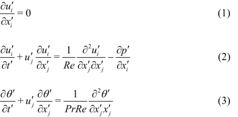
whereh，Ub， the flux-averaged exit mean scalar Θb， and their combinations are used to nondimensionalize the variables in the governing equations，′is the dimensionless instantaneous velocity，p′is the dimensionless instantaneous pressure，θ′is the dimensionless instantaneous scalar，Pr is the Prandtl number， andRe is the typical Reynolds number.

The governing equations are solved based on the fractional step method. The numerical code is developed based on the fully conservative fourth-order finite difference schemes for the fully staggered grid system，where the velocity or momentum variables are located on the cell face， meanwhile the scalar and pressure variables are stored in the cell center of the control volume， to avoid the discretization error owing to the oddeven decoupling between the velocity and the pressure，which would occur as the discretization of the partial differential flow equations is carried out in the grid system with co-located variables.

The central difference scheme is used for the spatial discretization of the governing equations； the temporal discretization is based on a hybrid implicit/explicit method， in which the implicit second-order Crank-Nicolson scheme is used for discretizing the viscous terms along the lateral direction and the third-order Runge-Kutta scheme is used for the discretization of other terms. The implicit treatment of the viscous terms is to eliminate the numerical viscous stability restriction， particularly for a low-Reynolds-number flow， which is similar to our cases. Moreover， the Poisson equation of the pressure is solved by the conjugate gradient method， which is the proper solution of partial differential equations. The accuracy of this code was verified by our previous work， a DNS of the canonical channel flow［16］.

2. Initial and boundary conditions

2.1 Initial condition

The flow condition at the jet origin is often called the initial condition， which mainly involves the exit Reynolds number， the nature of exit profiles of the mean velocity， and the exit turbulence intensity. In the present work， the attention will be focused on two factors， the Reynolds number and the mean velocity profile at the jet exit.

Re=2 000appears to be about the lowest value for the flow transition to turbulence at a rough entrance. We set two values for the exit Reynolds number，1 000 and 3 000， to capture the complete transition process to the fully-developed turbulence for the planar jet.

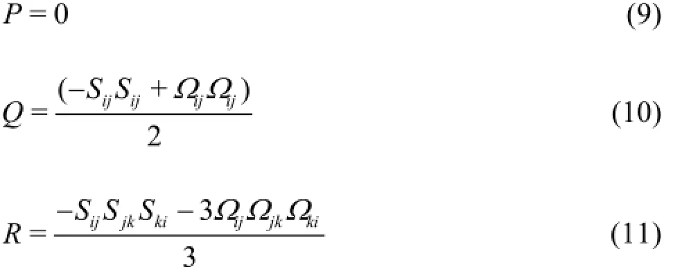
In order to resolve the flow motion in the smallest spatial scale （Kolmogorov microscale）， theoretically， the grid scale at each location should be smaller than the corresponding Kolmogorov microscale. Based on the empirical equation proposed by Friehe et al.［17］

whereηis the Kolmogorov microscale，Reis the exit Reynolds number， andx is the streamwise coordinate，ηis 0.047hat Re =1000and 0.021hat Re =3000at the location of （Lx′/2，0，0）in the computational domain. In consideration of the capacity of our computer， the grid numbers are set to be 356（x）×356（y）×80（z）for Re =1000and 756（x）×756（y）×160（z ）for Re =3000in the DNS.

Fig.2 Mean streamwise velocity profiles at the jet exit

For the planar jet， the mean velocity only contains the streamwise component at the jet exit. The exit profile of the mean velocity is associated with the jet nozzle type and the features of the inflow， which will be a sort of combinations of the top hat profile and the parabolic profile. In addition， the mean streamwise velocity profile of the fully-developed laminar channel flow along the direction of the channel height is in a parabolic shape. According to the above understanding， in the present DNS， two ideal and typical mean velocity profiles， i.e.， the top hat profile （TH） and the parabolic profile （PA）， are set at the jet exit and thesame mass flux is followed， as shown in Fig.2. Meanwhile， the experimental profiles from the work of Deo et al. are also shown in Fig.2， which were captured at the streamwise location of x/ h=0.5from the jet exit［11］.

The exit turbulence intensity is one percentile of the mean flow for the velocity field， which is randomly distributed. The exit mean scalar profiles are in the top hat shape， with the same scalar flux in all cases，and the exit turbulent scalar is zero. In the DNS，Pr is set to be 0.7， which is the typical value for air. A low co-flow is considered， where the ratio of the velocities between the low- and high- speed streams is 0.0599 in all cases， and it was proved that the jet transition to the self-similar state would be slowed down under this condition［18］.

2.2 Boundary conditions

The computational domain is a region truncated from the full physical domain. The boundary conditions should be appropriately chosen to close the difference between the flow in the numerical simulation and the real flow. Following the characteristics of the planar jet in an infinite or large physical domain， for the velocity variables， the lateral boundary condition is set as the Neumann boundary condition，=0， for the pressure and scalar variables， the Dirichlet boundary condition is used at the lateral boundary，p′=0 and θ′=0. One convective outflow condition， presented by Dai et al.［19］， is applied at the downstream exit，which was verified to introduce little error into the interior of the computation domain. Moreover， for all quantities the periodic boundary condition is imposed in the spanwise direction， where the planar jet is homogenous.

3. Velocity gradient tensor and its invariants

The dynamical behaviour of the velocity gradient tensor is important， which is closely related to the mechanism of the deformation of the fluid elements and in turn is related to the energy cascade process in the turbulence. This section focuses on the definition and the physical meaning of the invariants of the velocity gradient， the rate-of-strain and the rate-of-rotation tensors.

The velocity gradient tensor Aij=∂ui/∂xjcan be split into two components， i.e.， the symmetric Sijand the skew-symmetric Ωij， where Sij=（∂ui/∂xj+∂uj/∂xi）/2and Ωij=（∂ui/∂xj-∂uj/∂xi）/2are the rateof-strain and the rate-of-rotation tensors， respectively.

The characteristic equation for Aijis as follows：

where λiare the eigenvalues of Aij，P，QandR are the first， second， and third invariants of Aij， which are expressed as：

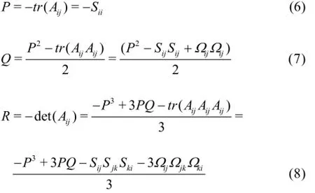
Under the condition of the flow incompressibility（P =0）， the invariants of Aijfor an incompressible flow takes the form：

whereQ can be divided into the strain component Qs=-SijSij/2， and the rotation component Qw=ΩijΩij/2， andR is composed of the strain component Rs=-SijSjkSki/3and -ΩijΩjkSki.

Following the above definitions for all parameters， the modulus of the second invariant of the rate-ofstrain tensor Qsis proportional to the local rate of the viscous dissipation of the kinetic energy ε=2nS2= -4nQs， where S2/2=SijSij/2is the strain product， the second invariant of the rate-of-rotation tensor Qwis proportional to the enstrophy density Ω2/2=ΩijΩij=2Qw， the modulus of the third invariant of the rate-of-strain tensor Rsis proportional to the strain skewness SijSjkSki. Moreover，-SijSjkSkiis a part of the production term in the strain product transport equation， which implies that a positive value of Rsis related to the production of the strain product， whereas a negative value of Rscorresponds to the destruction of the strain product.

The values of the invariants are independent of the orientation of the coordinate system and contain the information concerning the rates of the vortex stretching and rotation， and the topology and geometry of the deformation of the infinitesimal fluid elements. Based on the analyses of the invariants， the topology of the flow （enstrophy dominated versus strain dominated） or the enstrophy production （vortex stretching versus vortex compression） can be identified with the use of a relatively small number of variables， e.g.， the second and third invariants of the velocity gradient tensor.

Fig.3 Mean streamwise velocity profiles along the jet centerline

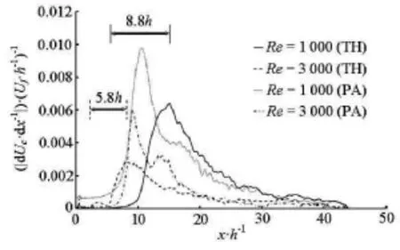
Fig.4 Decay rate of mean streamwise velocity along the jet centerline

Fig.5 Turbulent streamwise velocity profiles along the jet centerline

4. Results and discussions

4.1 DNS assessment

In this section， the flow development of the planar jet along the jet centerline is analyzed based on the streamwise profiles of the velocity and the scalar. Moreover， by making a comparison between our DNS results and the experimental data from the work of Deo et al.［11］， the accuracy of the DNS may be assessed. The data presented in this section will be calculated by averaging in time as well as across the homogeneous spanwise direction. The mean streamwise velocity profiles are shown in Fig.3， where Ucdenotes the mean streamwise velocity on the jet centerline，normalized by the mean streamwise velocity at the jet exit Uj， meanwhile， the decay rate of Uc，dUc/dx， is presented in Fig.4， normalized by Uj/h， in addition， the turbulent streamwise velocity profiles are shown in Fig.5， where urmscdenotes the root-meansquare （rms） streamwise velocity on the jet centerline， normalized by Uc.

The comparison between the cases of Re= 1000（TH）and Re=3000（TH）demonstrates the effects of the exit Reynolds number， in which the length of the jet potential core， the region where the mean streamwise velocity is equal to Uj（Uc/Uj=1）and without decay， is shortened with the increase ofRe ， when Re=3000（TH）， the fully-developed state is reached， with the constant turbulent intensity along the jet centerline （urmsc=constant）， sooner than when Re=1000（TH）， in the process of flow transition， between the potential core and the fully-developed state，the local maxima of the turbulent velocity and the decay rate of the mean velocity are located closer to the end of the potential core when Re=3000（TH），however， the values of these maxima are larger when Re=1000（TH）， as shown in Figs.4 and 5. The change in the exit mean velocity profile also affects the evolution of the streamwise velocity. One quite obvious observation is the decay rate of the mean velocity and the values of the local maxima of the turbulent velocity are larger in the case of parabolic profile.

Furthermore， one cannot ignore the fact that the cross-impact between the exitRe and the exit profile of the mean velocity causes the change in the effects of the single factor on the planar jet， for example， the effects of the exitRe with the exit parabolic profile differs from the counterparts with the top hat profile. It is observed that the length of the jet potential core is almost the same in the two cases of different exitRewith the exit parabolic profile. The cross-impact between all kinds of factors under the initial condition of the planar jet should be highlighted in the related researches.

Fig.6 Mean scalar profiles along the jet centerline

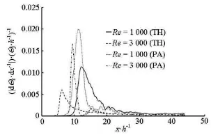
Fig.7 Decay rate of mean scalar along the jet centerline

Fig.8 Turbulent scalar profiles along the jet centerline

In the following part， the scalar field of the planar jet is studied. In analogy to the velocity field， Fig.6 shows the mean scalar profiles， where Θcdenotes the mean scalar on the jet centerline， normalized by the mean scalar at the jet exit Θj. Figure 7 presents the decay rate of the mean scalar （dΘc/dx）， normalized by Θj/h. Figure 8 shows the turbulent scalar profiles， where θrmscdenotes the turbulent scalar on the jet centerline， normalized by Θc.

In comparison with the velocity field， the scalar field reaches the fully-developed state faster， which means that the decay of the mean scalar becomes linear， and the turbulent scalar tends to be constant at a closer location to the jet exit. Meanwhile， we find that the overall magnitude and the local maxima of the turbulent scalar and the decay rate of the mean scalar are larger. These results can be attributed to the choice of Pr（=0.7）， as a higher scalar diffusion rate， compared to the viscous diffusion rate， is beneficial to the transition to the fully-developed state， which leads to a severer turbulent level in this process for the scalar field. Recalling the effects of the exitRe and the exit mean velocity profile on the velocity field， quite similar results are revealed for the scalar field， including the cross-impact of these two factors.

Fig.9 Sketch of the invariant map of （Qw，-Qs）

Fig.10 Typical invariant map of （Qw，-Qs）in fully developed jet［13］

The results from Deo et al.［11］at the exit Re= 1 500 and 3 000 are delineated in Figs.3 and 5. In their work， the length of the potential core at Re =3000is 5h， which is quite close to our result， meanwhile， the location for the mean velocity to attain the self-similarity is50hat Re =1500，20hat Re =3000， and 10hat Re=10 000in the streamwise direction. In our present results， the value is 23h at Re= 3000（TH）， greater than45hat Re =1000（TH），30hat Re=3000（PA）， and greater than45hat

Fig.11 Joint pdfs of （Qw，-Qs）

Re=1000（PA）， therefore， the comparison is reasonably well. In addition， the evolution and the magnitude of the turbulent velocity profiles also fit reasonably well， considering the difference of the exit mean velocity profile between the DNS and the experiment of Deo et al.， as shown in Fig.2.

4.2 Joint pdfs of the velocity gradient tensor invariants

In this section， the local topological characteristics of the joint pdfs of the invariants in the planar jet are studied in order to assess the evolution of the geometry of the flow motions along with the flow transi-tion. The approach taken in the DNS is to compute the second and third invariants of the velocity gradient，the rate-of-strain， and the rate-of-rotation tensors at each grid point in the flow. And then the joint pdfs of the invariants are calculated at three locations along the jet centerline，x/ h =0.5，x/ h =13.0and x/ h=37.0away from the jet exit. The computation of the joint pdfs at each location is based on the average of the values of the invariants at 5 000 time steps and 5（y）×5（z）grid points centered at the jet centerline.

4.3 Joint pdfs of （Qw，-Qs）

The invariant map of （Qw，-Qs）is shown in Fig.9， which can be used to analyze the geometry of the dissipation of the kinetic energy［13］. The horizontal line， defined by -Qs=0， represents the flow elements with high enstrophy but very small dissipation， as the solid body rotational dissipation at the center of a vortex tube. On the other hand， the vertical line， defined by Qw=0represents the flow elements with high dissipation but little enstrophy density， which corresponds to the flow elements containing a strong dissipation outside and away from the vortex tubes， as the irrotational dissipation. Moreover， the line angle is equal to 45owith the vertical and horizontal lines， where Qw=-Qs， and it represents the flow elements with high dissipation accompanied by high enstrophy density， which is consistent with the vortex sheet structures.

The typical invariant map of （Qw，-Qs）in the fully developed jet was presented in the work of Da Silva et al.［13］， as shown in Fig.10， where the contour levels are 0.01%， 0.03%， 0.1%， 0.3%， 1%， 3%， 10%，30%.

Figure 11 shows the joint pdfs of （Qw，-Qs）at three typical locations along the jet centerline under all four kinds of initial conditions， where the invariants are normalized by， the average of all sampling data at all typical locations， with the values of probability density varying from 0.01% to15.00%.

On the basis of the results for Re=1000（PA），firstly， we may see the differences of the geometry of the dissipation between the flow in transition and the fully developed turbulent flow. At the location of x/ h=0.5， which is close to the jet exit， the obvious tendency for all probability densities is observed to align with the vertical line defined by Qw=0， which attests a strong predominance of dissipation over enstrophy in this region for all scales of flow motion. Meanwhile， Qwtakes integrally a smaller value than Qs， which reveals the absence of the solid body rotation.

The flow at the location of x/ h =13.0witnesses larger values of Qw， which implies the growth of vortex tubes especially at the levels of small probability density， along with the flow transition. For the flow elements at the location of x/ h=37.0， the contour lines， associated with the most frequent values of Qwand Qs， see a tendency of aligning with the vertical line defined by Qw=0， however， the contour lines for most intense values of Qwand Qs， with small probability densities， show tendencies， aligning not only with the vertical line defined by Qw=0but also with the horizontal line defined by -Qs=0， which is different from the flow elements near the jet exit. Here，we find that the flow elements at this location show typical features of the fully developed region， as shown in Fig.10. The results point to a topology in the fully-developed planar jet where the vortex tubes， the vortex sheets， and the zones of irrotational dissipation all exist， but the irrotational dissipation with small velocity gradient dominates.

Fig.12 Sketch of the invariant map of （R， Q）

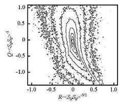
Fig.13 Typical invariant map of （R， Q）in fully developed jet［13］

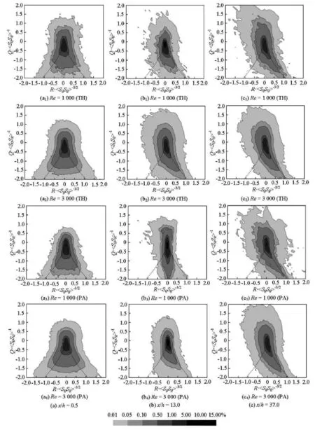
Fig.14 Joint pdfs of （R， Q）

Following the flow transition， the characteristics of the joint pdfs of （Qw，-Qs）indicate that in most cases of the flow domain velocity， the gradients assume small values， which can be confirmed by the fact that the largest values of the joint pdfs are around the origin， （Qw=0，-Qs=0）. In the downstream region of the planar jet， approaching to the fully-developed state， the vortex tubes with solid body rotation and little kinetic energy dissipation exist but as rare events. Moreover， as the exitRe increases from 1 000 to 3 000， the shape of the joint pdfs map at x/ h=13.0 and x/ h =37.0shows better similarity， which confirms the faster transition to the typical dissipation geometry in the fully-developed state of the planar jet. Meanwhile， the stronger tendency towards the irrotational dissipation at Re=1000（PA）supplies the answer to the nonzero mean velocity decay near the jetexit， as shown in Figs.3 and 4.

4.4 Joint pdfs of （R， Q）

On the basis of the definitions ofQandR， firstly， the sign ofQ illustrates the physical nature of the fluid elements. With positiveQ ， the enstrophy dominates over the strain product， whereas， with negativeQ ， the opposite situation happens. Secondly， after the sign ofQ is determined， the meaning ofRcan be inferred. If Q≪0，R≈Rs=-SijSjkSki/3， therefore， positiveR is related to the production of the strain product with the sheet structure， whereas， negativeR is related to the destruction of the strain product with the tube structure. If Q≫0，R≈-ΩijΩjkSki， positive Rimplies that the vortex is more in compression than in stretching， whereas， the vortex stretching is dominant with negativeR . The above four cases are shown in Fig.12［13］.

The （R， Q）map will assist us in analyzing the relation between the local flow topology （enstrophy or strain dominated） and the strain production term （vortex stretching or vortex compression）， which is associated with the geometry of the deformation of the fluid elements （contraction or expansion）.

The tent-like curve in Fig.12 is the DA=0line where DA=0is the discriminant of Aijgiven by

The typical invariant map of （R， Q）in a fully developed jet is shown in Fig.13［13］， where the contour levels are the same as in Fig.10.

The joint pdfs of （R， Q）obtained in our simulation are shown in Fig.14， where the invariants are also normalized by. The analysis of Fig.14 is also based on the condition of Re=1000（PA）. Close to the jet exit （x/ h=0.5）， the joint pdfs assume a symmetrical shape along the vertical line， defined by R= 0， with a narrow top and a wide bottom. The symmetrical distribution ofR implies the equilibrium between the vortex stretching and the vortex compression as well as between the tube structure and the sheet structure； in addition， the predominance of the strain product over the enstrophy can be observed as the joint pdfs below the horizontal line， defined by Q =0， which keeps a larger area.

In the transition process （x/ h=13.0）， the parts with small probability densities and intense values of RandQare firstly transformed into the characteristic teardrop shape in the fully developed jet， as shown in Fig.13， and the bottom part of the contours is transformed more obviously， which reveals the evolution of the vortex structure is faster than the evolution of the fluid elements deformation in the transition process of the planar jet.

When the flow arrives at the location of x/ h= 37.0， the （R， Q）map assumes the characteristic teardrop shape， where we can find the strong anti-correlation in the regions （R＞0，Q＜0） and （R＜0，Q＞0）. The teardrop shape represents the dominant sheet structure and enstrophy production by vortex stretching，which is at the core of the description of the turbulence energy cascade from the large scales to the small scales in the fully-developed turbulence.

In addition， we focus on the effects of initial conditions. The results of the joint pdfs of （R， Q）show that the flow transition is faster with a larger exitRe and under the condition of Re=1000（PA）the dissipation of kinetic energy is intenser. Moreover， another point might be made clearer here， that is， if we make a comparison between Re =3000（TH）and Re =3000（PA）at the location of x/ h =13.0，Q will take more large positive values and the shape is more similar between x/ h =13.0and x/ h =37.0at Re=3000（TH）， which implies that the top hat profile for the mean velocity at the jet exit will be beneficial to the transition of the local geometry and topology of the fluid elements in the planar jet.

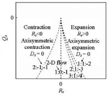
Fig.15 Sketch of the invariant map of （Rs， Qs）

Fig.16 Typical invariant map of （Rs， Qs）in fully developed jet［13］

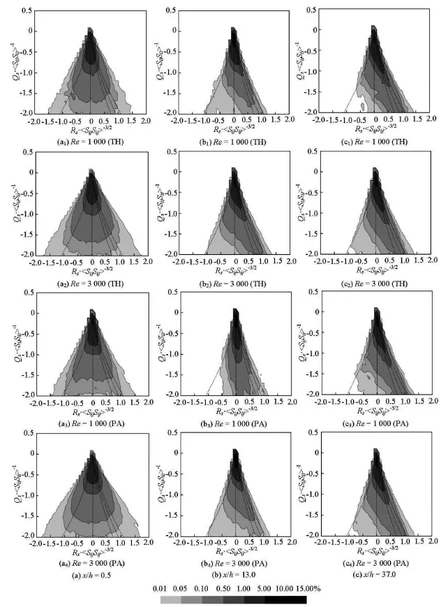
Fig.17 Joint pdfs of （Rs， Qs）-（1）

4.5 Joint pdfs of （Rs， Qs）

It is recalled that Rsand Qsare the third and second invariants of the rate-of-strain tensor Sij， respectively， which implies that the （Rs， Qs）map will be useful to analyze the geometry of the local straining （or deformation） of the fluid elements.

Since Qs=-ε/4n， the Qswith a large negative value is associated with an intense kinetic energy dissipation. In addition， the deformation of the fluidelement can be elucidated according to the sign of Rs， the positive value of Rsimplies the expansion of the fluid element， where the local straining is enhanced，whereas， the destruction of the strain product is associated with the negative value of Rs， which is followed by the contraction of the fluid element.

After defining αs，βsand γsto be the eigenvalues of Sij， ordered as αs≥βs≥γs，Rscan be written as -αsβsγs， and the sign of Rswill accord with the sign of βs. Due to the incompressibility，αs+ βs+γs=0， and hence Rs＞0implies that αs， βs＞0and γs＜0， whereas，Rs＜0implies that αs＞0and βs，γs＜0.

The invariant map of （Rs， Qs）is shown in Fig.15［13］， where five red dash lines are drawn on the basis of the discriminant of S，D=27/4R2+Q3，ijsssand the several typical values of the eigenvalues of Sij. Each line in the map is associated with a given flow geometry：αs：βs：γs=2：-1：-1（axisymmetric contraction），1：0：-1（two-dimensional flow），3：1：-4（biaxial stretching）， and 1：1：-2（axisymmetric stretching）［13］. The typical invariant map of （Rs， Qs）in the fully developed jet is shown in Fig.16［13］， where the contour levels are the same as Fig.10. This map shows that the most frequent values show a tendency toward the line （2：1：-3）， while the intermediate values seem to be closer to 1：1：-2.

Based on the joint pdfs of （Rs， Qs）in our simulation， shown in Fig.17， the geometry of the straining of the fluid elements is analyzed. Take the example of Re =1000（PA）， at the location of x/ h=0.5， the joint pdfs are symmetrical along the line （1：0：-1），which shows that the deformation of the flow elements has no preference here， and all shapes are with a wide bottom， which implies that a large dissipation dominates at all levels of the flow motion close to the jet exit.

The results at the location of x/ h=13.0show that， in the transition process of the planar jet， the transformation of the joint pdfs also starts from the contour line with the large probability density. And the expansion gradually predominates the contraction，meanwhile， the local straining is continually enhanced. In the downstream region （x/ h =37.0）， the （Rs， Qs） map shows a strong preference for the zone Rs＞0， Qs＜0， indicating a predominance of sheet structures， associated with expansive straining of the fluid elements， although the contractive straining also exists at some much fewer points. Figures 18 and 19 are shown as the supplement of Fig.17， and it can be observed that the most probable geometry of the fluid elements corresponds to a geometry between 3：1：-4（biaxial stretching） and 1：1：-2（axisymmetric stretching）， and the tendency changes from 3：1：-4to 1：1：-2along with the increase of the value of the joint pdf. For the effects of the exit Re， at the location of x/ h =0.5，Rstakes some larger value at a large exit Re， which indicates that a stronger contraction or expansion of the fluid elements occurs near the jet exit under this condition.

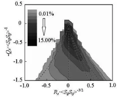
Fig.18 Joint pdfs of （Rs， Qs）-（2）

Fig.19 Joint pdfs of （Rs， Qs）-（3）

5. Conclusions

The DNS based on the finite difference method is carried out to simulate the flow transition in the planar jet. With the computation of several velocity and scalar variables and the invariants of the velocity gradient tensor， the present investigation provides some insights on the rates of vortex rotation and stretching， the topology and geometry of deformation of the fluid element， and the kinetic feature of the local straining. Based on these information， we compare the jet in the transition process with the fully developed turbulent jet， meanwhile， the effects of the exit Re and the exit mean velocity profile on the evolution of the planar jet are also studied.

The results reveal that in the jet potential core，the flow has a strong predominance of dissipationover enstrophy and the equilibrium between vortex stretching and vortex compression. In the transition process of the planar jet， the evolution of the vortex structure is faster than the evolution of the deformation of fluid elements， meanwhile the local straining is gradually enhanced. After the planar jet reaches the fullydeveloped state， the irrotational dissipation with small velocity gradient dominates， however， the vortex tubes with solid body rotation and little kinetic energy dissipation still exist with the small probability density，in addition， the characteristic teardrop shape of the（R， Q）map can also be observed， which implies the remarkable sheet structure and vortex stretching， the geometry of the fluid elements with the most frequent occurrence should be a geometry between biaxial stretching and axisymmetric stretching， as shown by the（Rs， Qs）map.

As the exitReincreases， the length of the jet potential core becomes shorter and the flow transition is promoted， however， the stronger turbulent variables are observed at the small exit Rein the flow development process. On the other hand， the parabolic profile for the exit mean velocity enhances the decay of the mean variables and the turbulent variables. Meanwhile， the cross-impact between the exitRe and the exit profile of the mean velocity causes the change of the effects of the single factor on the flow， especially in the near region of the jet. In addition， the large exitRe is obviously beneficial to the transition of the local topology and geometry of the planar jet to the fullydeveloped turbulent state.

Acknowledgements

This work was supported by the Collaborative Research Project of the Institute of Fluid Science，Tohoku University and supported by Grants-in-Aid（Grant Nos. 25289030， 25289031） from the Ministry of Education， Culture， Sports， Science and Technology in Japan.

［1］ GORDEYEV S. V.， THOMAS F. O. Coherent structure in the turbulent planar jet， Part 2： Structural topology via POD eigenmode projection［J］. Journal of Fluid Mechanics， 2002， 460： 349-380.

［2］ ATASSI O. V.， LUEPTOW R. M. A model of flapping motion in a plane jet［J］. European Journal of Mechanics B/Fluids， 2002， 21： 171-183.

［3］ DEO R. C.， MI J. and NATHAN G. J. The influence of Reynolds number on a plane jet［J］. Physics of Fluids，2008， 20（7）： 075108.

［4］ DEO R. C.， NATHAN G. J. and MI J. Comparison of turbulent jets issuing from rectangular nozzles with and without sidewalls［J］. Experimental Thermal and Fluid Science， 2007， 32（2）： 596-606.

［5］ DEO R. C.， MI J. and NATHAN G. J. The influence of nozzle aspect ratio on plane jets［J］. Experimental Thermal and Fluid Science， 2007， 31（8）： 825-838.

［6］ DEO R. C.， MI J. and NATHAN G. J. The influence of nozzle-exit geometric profile on statistical properties of a turbulent plane jet［J］. Experimental Thermal and Fluid Science， 2007， 32（2）： 545-559.

［7］ SURESH P. R.， SRINIVASAN K. and SUNDARARAJAN T. et al. Reynolds number dependence of plane jet development in the transitional regime［J］. Physics of Fluids， 2008， 20（4）： 044105.

［8］ TERASHIMA O.， SAKAI Y. and NAGATA K. Simultaneous measurement of velocity and pressure in a plane jet［J］. Experiments in Fluids， 2012， 53（4）： 1149-1164.

［9］ SHIM Y. M.， SHARMA R. N. and RICHARDS P. J. Proper orthogonal decomposition analysis of the flow field in a plane jet［J］. Experimental Thermal and Fluid Science， 2013， 51： 37-55.

［10］ SAKAKIBARA J. Plane jet excited by disturbances with spanwise phase variations［J］. Experiments in Fluids， 2013， 54（12）： 1-16.

［11］ DEO R. C.， NATHAN G. J. and MI J. Similarity analysis of the momentum field of a subsonic， plane air jet with varying jet-exit and local Reynolds numbers［J］. Physics of Fluids， 2013， 25（1）： 015115.

［12］ STANLEY S. A.， SARKAR S. and MELLADO J. P. A study of the flow-field evolution and mixing in a planar turbulent jet using direct numerical simulation［J］. Journal of Fluid Mechanics， 2002， 450： 377-407.

［13］ DA SILVA C. B. and PEREIRE J. C. F. Invariants of the velocity-gradient， rate-of-strain， and rate-of-rotation tensors across the turbulent/nonturbulent interface in jets［J］. Physics of Fluids， 2008， 20（5）： 055101.

［14］ WU N.， SAKAI Y. and NAGATA K. et al. Analysis of flow characteristics of turbulent plane jets based on velocity and scalar fields using DNS［J］. Journal of Fluid Science and Technology， 2013， 8（3）： 247-261.

［15］ ATKINSON C.， CHUMAKOV S. and BERMEJOMOREMO I. et al. Lagrangian evolution of the invariants of the velocity gradient tensor in a turbulent boundary layer［J］. Physics of Fluids， 2012， 24（10）： 105104.

［16］ SUZUKI H.， NAGATA K. and SAKAI Y. et al. Improvement of the DNS of turbulent channel flow using the finite difference method： Introduction of the compact scheme to the viscous terms for high spatial resolution in the dissipation range［J］. Transactions of the Japan Society of Mechanical Engineers Ser. B， 2009，75（752）： 642-649.

［17］ FRIEHE C. A.， VANATTA C. W. and GIBSON C. H. Jet turbulence： Dissipation rate measurements and correlations［C］. ANARD Conference Proceedings No.93 on Turbulent Shear Flows. London， UK， 1971.

［18］ HABLI S.， SAID N. M. and PALEC G. L. et al. Numerical study of a turbulent plane jet in a coflow environment［J］. Computers and Fluids， 2014， 89（2）： 20-28.

［19］ DAI Y.， KOBAYASHI T. and TANIGUCHI N. Large eddy simulation of plane turbulent jet flow using a new outflow velocity boundary condition［J］. JSME International Journal. Series B， Fluids and Thermal Engineering， 1994， 37（2）： 242-253.

* Biography： WU Nan-nan （1984-）， Male， Ph. D.， Lecturer