Weidong Jiang,Haowen Chen,and Xiang Li

College of Electronics Science and Engineering,National University of Defense Technology,Changsha 410073,China

Antenna geometry strategy with prior information for direction-nding MIMO radars

Weidong Jiang,Haowen Chen*,and Xiang Li

College of Electronics Science and Engineering,National University of Defense Technology,Changsha 410073,China

The antenna geometry strategy for directionnding (DF)with multiple-input multiple-output(MIMO)radars is studied. One case,usually encountered is practical applications,is considered.For a directional antenna geometry with a prior direction, the trace-optimal(TO)criterion(minimizing the trace)on the average Cram´er-Rao bound(CRB)matrix is employed.A qualitative explanation for antenna geometry is provided,which is a combinatorial optimization problem.In the numerical example section,it is shown that the antenna geometries,designed by the proposed strategy,outperform the representative DF antenna geometries.

multiple-input multiple-output(MIMO)radar,directionnding(DF),antenna geometry strategy,Cram´er-Rao bound (CRB),trace-optimal(TO),simulated annealing(SA)algorithm.

1.Introduction

Multiple-input multiple-output(MIMO)radars have attracted an increasing attention,where the term MIMO refers to the use of multiple-transmit as well as multiplereceive antennas.MIMO radars can transmit,via its antennas,multiple probing signals that may be correlated or uncorrelated with each other[1–3].There are two basic regimes of architecture considered in the current literature [2].One is called the statistical MIMO radar with widely separated antennas,which captures the spatial diversity of the target’s radar cross section(RCS)[3].This spatial diversity gain can improve the target detection and estimation of variations parameters.The other is called the coherent MIMO radar with colocated antennas,which can obtainextensionofthe apertureby virtualarraysandlarger degrees of freedom(DOF)to improve the target parameter estimation,parameter identiability and muchexibility for transmit beampattern design[1].Here,we discuss a colocatedMIMO radararchitecture,whichis a good directionnding(DF)system.

The waveformdesign strategies of MIMO radars,which aim to get larger DOF,have been extensively studied in existent literature for different given scenarios such as in [4–7].In this paper,we attempt to optimize the antenna geometry for DF MIMO radars.As in array signal processing,the antenna positions for a colocated MIMO radar stronglyaffect the targetdirectionestimation performance. Since the phases of the signals arrivingat receivers depend on the relative position of the target with respect to the antennas in far-eld scenes.Despite a rich direction estimation literature for MIMO radars[6],limited research has been dedicated to studying the effects of antenna geometry on direction estimation performance,while a majority of research has been focused on the direction estimation algorithms and their analytical performance bounds.Furthermore,very often,only the uniformlinear conguration [8–9]and its two-dimensional(2-D)extensions have specially been studied since they are easier to analyze and be adapted to fast implementations.

In this paper,we concentrate on the antenna geometries forDF MIMO radarswhich havethe optimaldirectionperformance[10–11]with a prior direction(such as an early warning radar,the prior information of the space angles can be obtained by the expert knowledge or statistical results.),under a given antenna constraint region.To assess the accuracy of the estimation,a standard mathematical tool is Cramer-Rao bound(CRB)[12].This bound is a lower bound on any(locally)unbiased estimators.So,the CRB is useful as a touchstone against which the efciency of the considered estimators can be tested.In[5,7,13],the expressions of CRB for direction parameters are derived for the colocated MIMO radar.However,the effects of antenna geometry on the direction estimation performance are not emphasized,and only the planar congurations are considered.In this paper,we will“borrow”the expression of CRB in[5],fordirectionparameterwith the antennapositions,while extend it to three-dimensional(3-D)cases,which is more appropriate to the practical applications.

For a directional antenna geometry design with a prior direction,we adopt minimizing the trace of the average (Bayesian)CRB matrix(referred to average trace-optimal (ATO))as a criterion,assuming that the direction parameters are the random variables with a prior probability distribution.The Bayesian CRB is a lower bound on the mean-squared error of the estimation of a random parameter and is independent of any particular estimator[14]. Then,it is a useful criterion for antenna geometry design. Because the antenna positions are nonlinear functions of the resulting cost criteria,the closed-formsolutions are not available except for a few special cases,thus we should employ nonlinear function minimization techniques.Here, thesimulatedannealing(SA)algorithm[15]is used,which has been considered as a good tool for complex nonlinear optimization problems and employed extensively in conventional antenna geometry design,such as in[16,17].

This paper is arranged as follows.In Section 2,we explain the measurement model for a DF MIMO radar and introduce the statistical assumptions.Section 3 gives the expression of CRB for direction parameters with the array positions.In Section 4,we dene the optimization problem and give the corresponding solution.In Section 5,we present some numerical examples to illustrate the superior performanceof the antenna geometry designed by the proposed strategy,comparing with the representative conguration.Finally,Section 6 concludes the paper.

Notation:In this paper,we use boldface lowercase letters forvectors and boldfaceuppercaseletters for matrices. We use{·}∗,{·}T,{·}Hand{·}−1for the complex conjugate,transpose,Hermitian transpose and inverse transpose of a matrix,respectively.Re{·}and Im{·}denote the real and imaginary parts,respectively.

2.Measurement model

Consideran MIMOradarsystem with Mttransmitand Mrreceive antennas,for which all the antennas are identical omnidirectional(see Fig.1).The transmit and receive antennas are located in a 3-D Cartesian coordinate system (x,y,z).Assume the transmit antennas are located at tk= [txk,tyk,tzk]T(k=1,...,Mt),and the receive antennas are located at rl=[rxl,ryl,rzl]T(l=1,...,Mr).Denote β=[t1,...,tMt,r1,...,rMr]Tas the antenna position matrix.The gravity centers of transmit and receive antennasareattc=[xtc,ytc,ztc]Tandrc=[xrc,yrc,zrc]T, respectively[18],given by

Fig.1 Illustration of colocated MIMO radar geometry

The set of transmitted signals expressed in low-pass equivalent form is given by1,...,Mt),where E is the total transmitted energy. Each of the waveform sk(t)is normalized and satiseswhere T is the observation interval. Then,the aggregate power transmitted by the transmitters is the constant E,regardless of the number of transmit antennas.Let xk[n](k=1,...,Mt;n=1,...,N)denote the discrete-time baseband signal transmitted by the kth transmit antenna,where n and N denote the sampled time and the number of snapshots of each transmitted signal pulse,respectively.

Let a point target be present in a resolution cell with coordinates p0=(x0,y0,z0).Let θ=[φ,ϕ]T∈Θ ≜[0,2π)×[−π/2,π/2]denote the direction parameter vector.φ andϕ are azimuth andelevation of the target towards all antennas,respectively.Then,using the received data model in[1,5]with a single target case,the data matrix can be written as

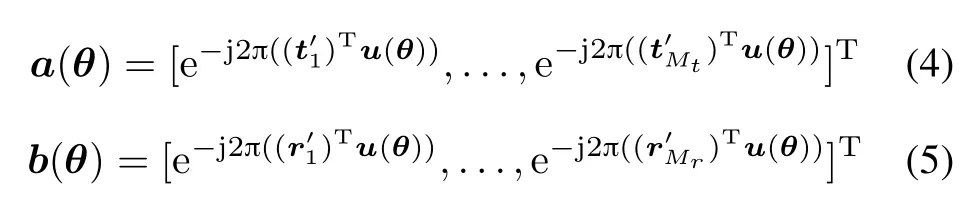
where the columns of Y ∈CMr×Nare the received data vectors,the rows of X ∈ CMt×Nare the transmitted waveforms,which are known and deterministic;ζ is the unknown target complex amplitude,which is proportional to the RCS of the target;Z∈CMr×Nis the interference andnoise term.For simplicity,we assume that the columns of Z are independent and identically distributed circularly symmetric complex Gaussian random vectors with zero mean and an unknown covariance matrix Q= σ2ZIMr, where IMrdenotes the Mrth-order identity matrix.Without loss of generality,we assume that X and Z are independent.And a(θ)and b(θ)are the steering vectors of thetransmit and receive antennas[19],respectively,given by

From(3),theunknownparameters,tobeestimatedfrom the data matrix Y,are ϑ=[Re{ζ},Im{ζ},θT]T.

3.Review of the CRB results in[6]

In this section,we present the CRB for target parameter vector ϑ based on the results given by[6].The Fisher information matrix(FIM)with respect to ϑ can be written as

wherethe notationsare givenby(7)–(12)with⊙denoting the Hadamard matrix product.

Thus the corresponding CRB matrix is

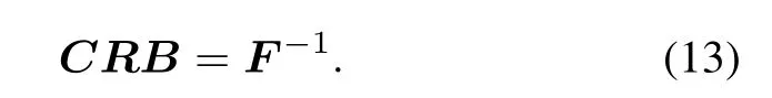
It is worth noting that the CRB matrix for ϑ depends not only on NRX,which contains the total transmit energies via each antenna and the correlations between transmit waveforms(thisisemphasizedin[5]),butalsoonthesteering vectors of the transmit and receive antennas,which contain the antenna geometry information.

4.Antenna geometry design under constraint region

In this section,we show the antenna geometry design for DF MIMO radars.Firstly,we assume that the antennas are constrained to lie in a closed,connected region DΓ⊂R3,which is bounded by a closed curve surface Γ.Let D=DΓ×···×DΓ⊂R3×(Mr+Mt)denote the constraint region for the antenna position matrix,thus

The following lemma will be useful in the optimal antenna geometry design under the constraint region.

Lemma 1The optimal antenna geometry lies on the antennaconstraintboundary,furthermore,the optimalcongurations have all antennas on the boundaryof constraint region Γ.

ProofSee[11]. □

Generally,we are interested in some area of the whole space.Giving an example,for the air surveillance radar withexibly distributed arrays[20],the whole airspace should be searched atrst.However,when some special space is chosen,the proposed algorithm as following can be utilized for heightening the performance of target parameter estimation.The prior probability distribution of direction parameters,written by f(φ,ϕ),can be obtained, then the optimal antenna geometry is no longer isotropic [21].First,consider minimizing the trace of the average CRB matrix with antenna position matrix,which is referred to the ATO criterion,

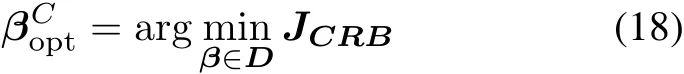
where CRB(φ)and CRB(ϕ)are respectively the CRB variances of the azimuth and elevation,both of which include the positions of all antennas.

Forgeneralboundariesorpriorprobabilitydensityfunctions,usually,it is impossible tond an analytic solution for the optimization problems in(18).From Lemma 1,the optimal geometries have all antennas on the boundary of the constraint region.As a result,the dimension of the design optimization in(18)is reduced from 3(Mt+Mr) to 2(Mt+Mr).Then the optimal solution is found as a 2(Mt+Mr)-dimensional search for antenna positions. Specially,if the constraint region DΓis convex,the optimal solution can be solved efciently using interior point methods[22].It is worth noting that the interior point methods cannot be used if the problem does nott into its convex framework.Hence,more general methods are needed for solving problems that arise in practice.Genetic algorithms[23]and algorithms based on physical processes such as particle swarm optimization(PSO)[24] and simulated annealing(SA)[15]are capable of solving problems that are very general.The solution of(18)based on the SA algorithm will be given in the following.

The SA algorithm,which was initially developed for very large scale integration(VLSI)circuit design by Kirkpatrick et al.[15],exploits an analogy between the search for a minimum cost function and the physical process by changing a state while minimizing its energy.It has since evolved to be a powerful computational tool in multivariable optimization for a wide range of engineering problems,such as in[25].The major advantage of the SA algorithm over the traditional“greedy”optimization algorithms is the ability to avoid becoming trapped in local optima during the search process.The solution of(18)based on the SA algorithm will be illustrated in detail as follows. For the consistency with the assumption of Section 4,we assume that all the antennas(including Mttransmit antennas and Mrreceive antennas)are located on the boundary of the circular constraint region(with the diameter 2L) in 2-D cases.The similar solution can be extended to 3-D cases.

For the circular constraint region,we can use the polar coordinates L and δm(m=1,...,Mr+Mt)denoting the locations of the antennas conveniently,and the location of each antenna can be given by[Lcosδm,Lsinδm]Twith 0≤ δm＜ 2π.Let δ be a vector in RMr+Mtand (δ1,...,δMr+Mt)its components.Then the solution of (18)can be rewritten as

Our SA algorithm for the optimal antenna geometry is schematically shown in Fig.2.A detailed description of this algorithm is as follows.

Fig.2 Flowchart for designing optimal antenna geometry using SA

Step 0(Initialization):Choose

a starting point δ0;

a starting step vector v0;

a starting temperature T0;

a terminating criterion ε and a number of successive temperature reductions to test for termination Nε;

a test for step variation NSand a varying criterion c;

a test for temperature reduction NTand a reduction coefcient ρ.

Set i,j,k and l to 0.i is the index denoting successive point,j denotes successive cycles along every direction, k describes successive step adjustments,and l covers successive temperature reductions.Set h to 1.h is the index denoting the direction along which the trail point is generated,starting from the last accepted point.

Compute E0=E(δ0).

Setthebestpointreachedasδopt=δ0,andthebestcost function Eopt=E0

Set nu=0,u=1,...,Mr+Mt.

Set E∗u=E0,u=0,−1,...,−N∈+1.

Step 1Starting from the point δi,generate a random point δ′along the direction h:

where r is a random number generatedin the range[−1,1] by a pseudorandom number generator;ehis the vector of the hth coordinate direction;and vkhis the component of step vkalong the same direction.

Step 2If the hth coordinate of δ′lies outside the denition domain of E,i.e.,δm＜0 or δm≥2π,then return to Step 1.

Step 3Compute E′=E(δ′).

If E′≤Ei,then accept the new point.

Set δi+1=δ′and Ei+1=E′.Add 1 to i,and add 1 to nh.

if E′≤Eopt,then set

δopt=δ′and Eopt=E′.

end if;

else if E′＞Eiaccept or reject to the point with acceptance probability p according to the Metropolis criterion [26]:

where ΔE=E(δ′)−E(δi)and Tlis a parameter called temperature for the lth iteration.

Step 4Add 1 to h.If h≤Mr+Mt,go to Step 1;else set h to 1 and add 1 to j.

Step 5If j＜Ns,go to Step 1;else update the step vector vm.For each direction u the new step vector component v′uis The aim of these variationsin step length is to maintain the average percentage of accepted moves at about one-half of the total number of moves.The cuparameter controls the step variation along each uth direction.

Set vm+1=v′,j to 0,nuto 0(u=1,...,Mr+Mt), and add 1 to k.

Step 6If l＜NT,go to Step 1;else,it is time to reduce the temperature Tl:set Tl+1=ρTl,where ρ is smaller but very close to 1 and is chosen to be 0.95 in this design.Setand add 1 to l,set k to 0.

Step 7(Terminating criterion)If

then stop the search;else,add 1 to i,set δi=δopt,set Ei=Eopt.Go to Step 1.

It is worth noting that the step variation NSdecides the precisionof the optimumantenna locations.The larger NSbrings the better precision of antenna locations while the more iterative times.Reasonable values,found after some test optimizations,of the parameters that control the SA are

5.Numerical examples

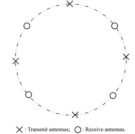
Fig.3 Isotropic antenna geometry with circular constraint region (Mt=Mr=4)

In this section,we compare the performance between the optimal antenna geometries designed in this paper and the representative one,isotropic antenna geometry,see Fig.3. The locations of transmit and the receive antennas are given by tk=[Lcosαk,Lsinαk]T(k=1,...,Mt)and rl=[Lcosβl,Lsinβl]T(l=1,...,Mr),respectively,where αk= 2π(k−1)/Mt+α0and βl= 2π(l−1)/Mr+β0with the initial phases α0and β0,respectively,tc=rc=[0,0]T.For convenience and fairness of comparisons,we assume that all antennas and the target(s)areonthe sameplane(onlyazimuthangle(s)).For the sake of simplicity,assume that both the transmit antennas and the receive antennas are located in the same circular constraint region with the diameter 2L,i.e.,the antenna positions are

Assume that a prior direction is given by the probability distribution shown in Fig.4(a),which represents a scenario where the radar system can detect for any direction, but it is expected that the target is primarily over a particular sector.Consider a four-transmit four-receive MIMO radar system.Fig.4(b)shows the ATO geometrysearching by the SA algorithm,which is different from the isotropic antenna geometry with equally spaced antennas.Thus,the ATOgeometryis notisotropicwhilehas thelargeraperture over the interested direction than other areas.

Fig.4 Optimal antenna geometry for the circular constraint region under a prior direction(1)

Similar to Fig.4,Figs.5(b)and 6(b)are the ATO geometries corresponding a prior direction as Figs.5(a)and 6(a),respectively.Fig.6 shows the performance,normalized by the performanceof the isotropic optimumantenna conguration in Fig.3,comparisons between the ATO geometries with the isotropic geometry versus the azimuth. It can be seen from Fig.7 that the performance of the geometries both in Figs.4(b),5(b)and 6(b)is superior to the one of the isotropic antenna geometry over the prior direction region,while is inferior in other directions,where the performancedescendsveryfast,especially for geometryin Fig.5(b).The reason is that only the narrower directionregion is focused on,then the performance of other regions is ignored.

Fig.5 Optimal antenna geometry for the circular constraint region under a prior direction(2)

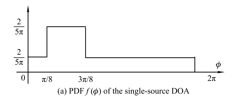
Fig.6 Optimal antenna geometry for the circular constraint region under a prior direction(3)

Fig.7 Azimuth estimation performance comparison with different antennas geometriesand)

Owing to the probabilistic nature of SA,different temperature schedulings and random initial geometries may lead to different results.However,if a logarithmic scheduling is chosen,almost all the process runs give slightly different results in terms of both energy values and antenna positions[15].This means that the resulting antenna geometry is stable and close to the optimal one.

6.Conclusions

The improvement of DF performance related to MIMO radars with colocated antennas can be explained as:the proposed methods allow one to minimize the performance bounds,given the numberof transmit/receiveantennas and the antenna constraint region,to optimize the antenna geometry.For an optimal direction antenna geometry with a known prior direction,we employe the ATO criteria and provide a qualitative explanation for antenna geometry design.

In practical application,there are many factors involved in the choice of the antenna geometry for MIMO radars.It is obviousthat the antenna geometrystrategy is greatly decidedby the mission of the radar system.We may get completely different antenna geometries under different design criteria.Many inspired results can be“borrowed”from conventionalarraysignalprocessingtotheantennageometry design of MIMO radars.This will be further studied in the near future.

Acknowledgment

The authors are very grateful for the insightful comments and suggestions made by the anonymous reviewers.

[1]H.W.Chen,X.Li,W.D.Jiang,et al.MIMO radar sensitivity analysis of antenna position for directionnding.IEEE Trans. on Signal Processing,2012,60(10):5201–5216.

[2]H.W.Chen,X.Li,H.Q.Wang,et al.Performance bounds of directionnding and its applications for multiple-input multiple-output radar.IET Radar,Sonar&Navigation,2014, 8(3):251–263.

[3]H.W.Chen,Y.Chen.Extended ambiguity function for bistatic MIMO radar.Journal of Systems Engineering and Electronics, 2012,23(2):195–200.

[4]D.R.Fuhrmann,G.S.Antonio.Transmit beamforming for MIMO radar systems using signal cross-correlation.IEEE Trans.on Aerospace and Electronic Systems,2008,44(1):71–186.

[5]J.Li,L.Xu,P.Stoica,et al.Range compression and waveform optimization for MIMO radar:a Cramer-Rao bound based study.IEEE Trans.on Signal Processing,2008,56(1):218–232.

[6]X.H.Wu,A.A.Kishk,A.W.Glisson.MIMO-OFDM radar for direction estimation.IET Radar Sonar&Navigation,2010, 4(1):28–36.

[7]I.Bekkerman,J.Tabrikian.Target detection and localization using MIMO radars and sonars.IEEE Trans.on Signal Processing,2006,54(10):3873–3883.

[8]W.Roberts,L.Z.Xu,J.Li,et al.Sparse antenna array design for MIMO active sensing applications.IEEE Trans.on Antennas Propagation,2011,59(2):846–858.

[9]R.Boyer.Performance bounds and angular resolution limit for the moving colocated MIMO radar.IEEE Trans.on Signal Processing,2011,59(4):1539–1552.

[10]H.Gazzah,S.Marcos.Cramer-Rao bounds for antenna array design.IEEE Trans.on Signal Processing,2006,54(1):336–345.

[11]U.Oktel,R.L.Moses.A Bayesian approach to arrary geometry design.IEEE Trans.on Signal Processing,2005,53(5): 1919–1923.

[12]P.Stoica,R.L.Moses.Spectral analysis of signals.Upper Sad-dle River,NJ:Prentice-Hall,2005.

[13]N.H.Lehmann,E.Fishler,A.M.Haimovich,et al.Evaluation of transmit diversity in MIMO-radar directionnding.IEEE Trans.on Signal Processing,2007,55(5):2215–2225.

[14]H.L.Van Trees.Detection,estimation,and modulation theory, part I.New York:Wiley,2001.

[15]S.Kirkpatrick,C.D.Gelatt,M.P.Vecchi.Optimization by simulated annealing.Science,1983,220(4598):671–680.

[16]P.Chen,Y.Y.Zheng,W.Zhu.Optimized simulated annealing algorithm for thinning and weighting large planar arrays in both far-eld and near-eld.IEEE Journal of Oceanic Engineering,2011,36(4):658–664.

[17]V.Murino,C.S.Regazzoni.Synthesis of unequally spaced arrays by simulated annealing.IEEE Trans.on Signal Processing,1996,44(1):119–122.

[18]D.H.Johnson,D.E.Dudgeon.Array signal procesing:concepts and techniques.Englewood Cliffs,NJ:Prentice-Hall, 1993.

[19]H.W.Chen,X.Li,Z.W.Zhuang.Antenna geometry conditions for MIMO radar with uncoupled direction estimation.IEEE Trans.on Antennas and Propagation,2012,60(7): 3455–3465.

[21]H.W.Chen,X.Li,Z.W.Zhuang.Performance bounds of directionnding and its applications for multiple-input multipleoutput radar.IET Radar,Sonar&Navigation,2014,8(3): 251–263.

[22]S.Boyd,L.Vandenberghe.Convex optimization.Cambridge, U.K.:Cambridge University Press,2004.

[23]R.L.Haupt,S.E.Haupt.Practical genetic algorithms. NewYork:Wiley,2004.

[24]J.Kennedy,R.C.Eberhart,Y.Shi.Swarm intelligence.San Francisco,CA:Morgan Kaufmann,2001.

[25]E.H.L.Aarts,P.J.M.V.Laarhoven.Statistical cooling:ageneral approach to combinatorial optimization problems.Philips Journal of Research,1985,40(4):193–226.

[26]N.Metropolis,A.Rosenbluth,A.Teller,et al.Equation of state calculations by fast computing machines.Journal of Chemical Physics,1953,21(6):1087–1090.

Biographies

Weidong Jiang was born in 1968.He received his B.S.,M.S.and Ph.D.degrees from the National University of Defense Technology, Changsha in 1991,1997 and 2001,respectively. He is currently a research fellow at the Research Institute ofSpace Electronics Information Technology in Electronics Science and Engineering School,National University of Defense Technology.Since 2003,he has been in the Research Institute of Space Electronics Information Technology where he focuses his interest on target recognition and radar signal processing.

E-mail:jwd2232@vip.sina.com

Haowen Chen was born in 1981.He received his B.S.degree in communications engineering from Engineering University of Air Force,Shanxi,China, in 2004,and M.S.E.E degree from National University of Defense Technology,Changsha,China,in 2007.He is currently pursuing his Ph.D.degree in electrical engineering from National University of Defense Technology.His research interests lie in the area of statistical signal processing,including sensor array signal processing,MIMO radar systems,MIMO radar signal processing,and radar target recognition.

E-mail:chenhw@nudt.edu.cn

Xiang Li was born in 1967.He received his B.S. degree from Xidian University,Xi’an in 1989,and M.S.and Ph.D.degrees from the National University of Defense Technology,Changsha in 1995 and 1998,respectively.He is currently a professor at the Research Institute of Space Electronics Information Technology in Electronics Science and Engineering School,National University of Defense Technology. In 1999,he joined the Key Lab of Automatic Target Recognition where he worked in the areas of radar system design,nonlinear signal processing and radar target recognition.Since 2003,he has been in the Research Institute of Space Electronics Information Technology where he focuses his interest on target recognition,signal detection and SAR imaging.

E-mail:lixiang01@vip.sina.com

10.1109/JSEE.2015.00054

Manuscript received July 04,2013.

*Corresponding author.

This work was supported by the National Natural Science Foundation of China(61072117;61302142).