MUSUMECI Rosaria E.， MARLETTA Vincenzo， ANDÒ Bruno， BAGLIO Salvatore， FOTI Enrico

1. Department of Civil Engineering and Architecture， University of Catania， Catania， Italy，E-mail： rmusume@dica.unict.it

2. Department of Electric， Electronic and Computer Science Engineering， University of Catania， Catania， Italy

Ferrofluid measurements of bottom velocities and shear stresses*

MUSUMECI Rosaria E.1， MARLETTA Vincenzo2， ANDÒ Bruno2， BAGLIO Salvatore2， FOTI Enrico1

1. Department of Civil Engineering and Architecture， University of Catania， Catania， Italy，E-mail： rmusume@dica.unict.it

2. Department of Electric， Electronic and Computer Science Engineering， University of Catania， Catania， Italy

（Received October 9， 2014， Revised November 3， 2014）

A novel direct measurement strategy of bottom velocities and shear stresses based on the use of ferrofluids is presented. Such a strategy overcomes some of the limits of state-of-the-art instruments. A preliminary experimental campaign has been carried out in the presence of currents in steady flow conditions in order to test the effects of ferrofluid quantity and of the controlling permanent magnetic force. An alternating current （AC） circuit and a direct current （DC） conditioning circuit have been tested. For velocities larger than 0.05 m/s， the near-bottom velocity-output voltage calibration curve has a monotone parabolic shape. The sensitivity of the instrument is increased by a factor of 30 when the DC circuit is used.

magnetofluids， Rosensweig effect， flow resistances， bed shear stresses， bottom velocities

Introduction

In physical modelling of hydraulic processes，measurements of wall shear stresses are extremely important. Indeed large flow resistances develop right at the boundaries， strongly affecting both the hydrodynamics and， in the presence of mobile beds， the sediment transport.

In the past， several instruments have been developed and used to measure the shear stresses generated at the bottom in the presence of waves and currents，such as mechanical shear plates or cells located at the bottom， thermal anemometry based on the use of hotfilm and hot-wire probes， acoustic and optic methodologies， such as ADV， LDA， PIV and PTV［1-4］or unconventional approaches such as bioluminescence［5］. However， the applications of most of such techniques are affected by several limits. For example， mechanical probes can provide only integral measures over areas of O （1 dm2）. Thermal probes， which represent the state-of-the-art for measuring bed shear stresses，are extremely sensitive to the operating conditions， e.g. they cannot be effectively used in the presence of impurities or sediments without damaging the probes. Finally， the widely spread optoacoustic instruments do not provide very accurate velocity measurements at the wall， due to the bottom-induced reflection.

Only very recently a new methodology for the measurement of the bottom shear stresses in a quasinoninvasive manner based on the use of ferrofluids has been qualitatively tested in the presence of an oscillatory motion［6］.

Ferrofluids are two-state systems made up by small ferromagnetic particles （with size 1 nm-15 nm）dispersed in an organic non-magnetic solvent［7］. A surfactant covers the nano-particles in order to prevent their agglomeration， which would be otherwise induced by the Van Der Waals forces and the magnetic forces. Although their name seems to suggest the opposite， the ferrofluids are superparamagnetic materials. Indeed， thanks to the nano-scale size of the dispersed particles， remaining at the fluidic state， the ferrofluids are deformed by the application of a magnetic field. Such a deformation disappears as soon as the magnetic field is removed. At the microscopic scale， long chains of particles are formed in the direction of the magnetic field， whereas at the macro-scale a series of spikes aligned along the magnetic field appears. Such a phenomenon is called “the Rosensweig effect”.

Thanks to their properties， the ferrofluids are used in a number of applications， ranging from mechanics， as lubricants or packings， to biomedics，where they are used in the drug targeting to magnetically drive the drug within the body. Several applications have been developed also in the field of optics and electronics， such as transducers or inertial sensors based on ferrofluids［8-12］.

In the present work， starting from the seminal work of Andò et al.［6］where a qualitative uncalibrated demonstration of the technique was presented， the magneto-rheological characteristics of ferrofluids are systematically exploited to propose a new quasi-noninvasive methodology for the measurement of the bottom velocities and shear stresses due to a steady turbulent current flow in the presence of a smooth bottom. In particular， an inductive read-out strategy is developed to transfer the movement of the ferrofluid into a voltage output signal， and two different conditioning circuits， a simpler alternating current （AC） and a more complex direct current （DC）， are tested to optimize the sensitivity of the proposed measurement methodology. An experimental calibration of the system is carried out in a small-scale highly controllable steady-current flume and the range of applicability of the proposed system is assessed and discussed.

1. Physical properties of ferrofluids

According to a series of previous experimental results， Odenbach［13］proved that the formation of structures of magnetic nano-particles has a significant influence on the magnetoviscous behavior of ferrofluids. By means of a mathematical model， Zubarev and Iskakova［14］showed that the formation of two types of structures， namely micro-chains of particles and drop bulk structures， plays an important role in controlling the rheological properties of ferrofluids.

Ferrofluids are also called magneto-rheological fluids， since their viscosity changes as a function of their level of magnetization. Roszkowski et al.［15］experimentally observed the presence of three regimes：（1） for a magnetic induction B＜1.4 mT the viscosity decreases as B increases， （2） for 1.4 mT＜B＜8.5 mT the viscosity increases as B increases in the range 5 Pa·s -9 Pa·s （i.e.， about 5 000-9 000 times the viscosity of water at 20oC）， （3） for 8.5 mT B＞ the viscosity abruptly increases due to the partial clogging of the capillary used in the experiments of Roszkowski et al.［15］.

Concerning the surface tension， by experimentally investigating the interfacial stability of a ferrofluid，it has been found that the surface tension can be assumed as a constant property， although in principle it should depend on the thermodynamic and magnetization characteristics. In particular for the air-ferrofluid interface the mean surface tension is equal to 0.0275 N/m， whereas at the water-ferrofluid interface the mean value is 0.0173 N/m. As regards the dynamic behavior of ferrofluids， it is recognized that such materials can be considered Newtonian fluids in the absence of a magnetic field and non-Newtonian fluids when they are magnetized.

In particular， if the magneto-particle distribution in the ferrofluid mixture is such that chain-like structure can be formed （i.e.， if the particle diameter is larger than a critical diameter） a yield stress exists，which increases with the number of strongly interacting large particles and it is proportional to the square of the applied magnetic field strength. In any case， the values of such a yield stress results relatively small，less than 0.07 N/m2， for a quite large range of magnetic fields （0 kA/m-80 kA/m）.

2. The proposed methodology

The proposed measuring technique is based on the idea that in the presence of a flow， a small quantity of ferrofluid （order of few thousandths of milliliters）positioned at the wall and controlled by the action of a permanent magnetic field， will deform not only because of the applied magnets， but also due to the flow which acts on the ferrofluid drop. More in details， in hydrostatic conditions， i.e. when only the magnetic field is present， due to the Rosensweig effect and to the tiny amount of ferrofluid， a single spike is formed，having the shape of a small cone， whose height is about 0.001 m （see Figs.1（a） and 1（c））. In dynamic conditions， such a cone will deform and will move in the flow direction as a consequence of the applied bottom shear stress （see Fig.1（b））.

Fig.1 Sketch of the ferrofluid spike

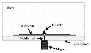
Fig.2 Sketch of the measuring system within the flume （ferrofluid height O （0.001m）， coils diameter 0.023 m）

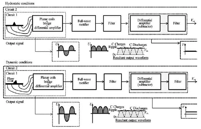
Fig.3 Schematic of the conditioning circuits （Circuit 1 and Circuit 2） and representation of the AC and DC output signal， both in static and dynamic conditions. Positioning of the ferrofluid spike within the flume

Therefore by detecting the displacement of the center of mass of the ferrofluid drop it should be possible to measure the bottom velocity or the bottom shear stress. In the present work， an inductive readout strategy to detect and quantify such a displacement is proposed and discussed.

Considering the sketch shown in Fig.2， one or more permanent magnets are used to generate the spike by exploiting the Rosensweig effect and to maintain the position of the ferrofluid drop at the measuring station. A metallic nail has been used to concentrate the magnetic field produced by the permanent magnets in order to obtain a single ferrofluid spike.

The inductive readout strategy makes use of two planar coils located at the bottom of the flume （see Fig.2）. The ferrofluid spike sits initially at the center of the two coils. The movement of the ferrofluid spike produces a variation of the magnetic permeability μ and consequently a variation of the inductance L in the coils. Therefore the displacement can be sensed by two planar coils， since the perturbation of the magnetic field generated by the displacement of the spike is transformed into a voltage change by a conditioning circuit which is connected to the coils in a differential configuration.

More in details， the conditioning circuit is made up by several components （see Fig.3）： （1） an initial alternating current （AC） bridge and a differential amplifier （Circuit 1）， （2） a full wave rectifier and a filter， （3） a differential amplifier which acts as a subtractor and a filter （Circuit 2）.

The output of the first part of the system （Circuit 1） is an alternating （sinusoidal） voltage signal， whose amplitude is proportional to the displacement of the ferrofluid drop （see Fig.3）. Then， the sinusoidal signal is rectified， by considering the absolute value of the voltage output. Finally a direct current （DC） signal is obtained by means of the subtractor and of the last filter （Circuit 2）.

In the present work both the results obtained by the first stage of the conditioning circuit （Circuit 1）and of the complete circuit， including the full wave rectifier and the consequent filters and subtractors （Circuit 2） are presented. It is worth pointing out that， by using Circuit 1， since the signal is generated at 100 kHz， the sampling frequency has to be very high（higher than 2 MHz）.

It follows that an important computational effort for the storage and the analysis of the data is required in this case. In order to facilitate the recording and the analysis of the results， the second and third stages were added to Circuit 2 to have a filtered DC output signal （see Fig.3）， which allows much lower sampling frequencies， O（1kHz）.

3. Hydrodynamics around the ferrofluid spike

The hydrodynamics which occurs around the fe-rrofluid spike in the presence of an external steady current is quite complex. Indeed， it must be considered that： （1） the ferrofluid has a conical shape and （2） it remains at the liquid state. Therefore， when deformed and misplaced by the action of an external flow， not only the ferrofluid spike is characterized by a changing three-dimensional shape， but also for the sake of velocity continuity at the surface the ferrofluid itself should circulate within the liquid drop， while its macroscopic position is dynamically controlled by the equilibrium between the applied magnetic field and the force exerted by the external flow.

Notwithstanding the complexity of the problem，some information on the flow conditions is discussed here by considering similarities with well-known type of flows， such as rigid circular cylinders， spheres，cones， and liquid spherical drops.

First of all， the ferrofluid can be viewed as an obstacle to the flow and separation of the boundary layer may occur， depending on the flow characteristics. As a first approximation， the flow around the ferrofluid spike can be considered similar to the flow around a rigid smooth cylinder. The local Reynolds number of the ferrofluid drop is defined as

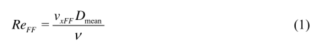
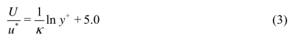
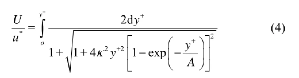
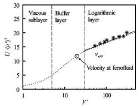
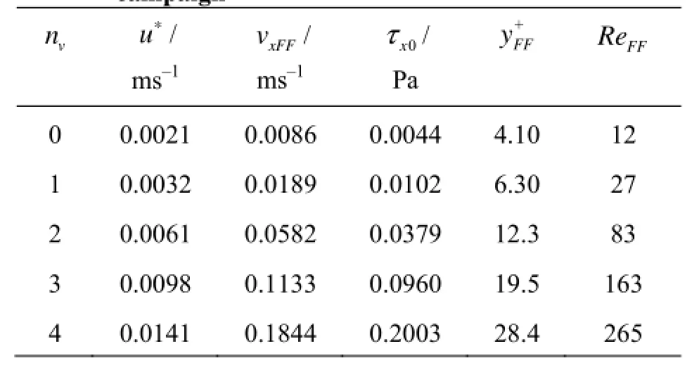
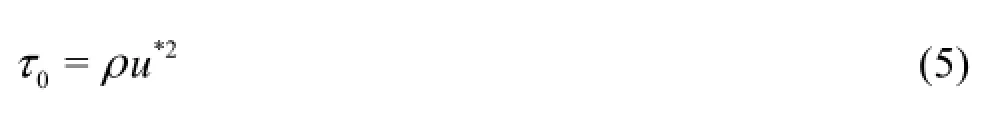
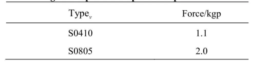
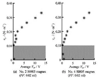
wherexFFv is the velocity of the external flow upstream of the ferrofluid drop，meanD is the mean diameter of the ferrofluid assumed constant in analogy with the cylinder case， and ν is the kinematic viscosity of water. A separation of the boundary layer over the cylinder surface should occur as follows： if 5< ReFF＜40， a fixed pair of symmetric vortices is present on the lee side of the ferrofluid， if 40

If vortices are shed due to the presence of the ferrofluid， a Strouhal number can be defined as

wherevf is the vortex shedding frequency andxV is the velocity of the outer flow. For small Reynolds numbers， St is constant and equal approximately to 0.2.

From the dynamic point of view， the flow around the ferrofluid spike exerts a resultant force on the spike itself， such a force is due to two contributions：one from pressure， i.e.， the pressure drag or form drag，and one from friction， i.e.， the friction drag. The drag coefficientDC on a circular cylinder is a monotonic decreasing function of the Reynolds number. The presence of turbulence in the incoming flow tends to stabilize the value of the mean drag coefficient even at low Reynolds number. Indeed in the case of a rigid cylinder， the contribution of friction is often neglected，while ratio between friction （on the surface of the structure） and the form drag decreases as the Reynolds number increases （for Re smaller than 105）. In any case， for Reynolds numbers larger than 104the contribution of friction on the surface of the body is about 2%-3% of the drag coefficient.

Since the ferrofluid has a conical shape， its threedimensionality should also be taken into account. First of all， in the case of 3-D obstacle transition to turbulence should occur earlier compared to the cylinder case. For example， in the case of a sphere，cirtRe is about 5×105， whereas it is 106in the case of a cylinder.

Literature experimental results on the flow past a rigid smooth cone placed on a flat plate， considering cones with different angle at the vertex （60o， 90o，120o， 180o） have shown that， for vertex angle of the cone smaller than 120o， the pressure distribution is similar to that on a circular cylinder and it has a peak in the proximity of the base of the cone， showing a negative pressure gradient， which indicates the presence of a necklace vortex around the cone. Moreover， it has been also found that the log wall law holds both inside and outside of the wake region. In particular， outside of the wake region， the results are those of the boundary layer on a flat plate， inside the wake region and close to the wall， where the log wall law holds， there is a larger velocity defect （larger velocity compared to the outer flow） due to the negative wake effect. The local drag coefficient at several heights along the cone surface， namedDzC， decreases as the vertex angle increases and has a maximum at levels z/ H=0.1-0.2. For example， in the case of a cone with a vertex angle equal too60， the maximum value is about 0.8， whereas the minimum value at the vertex is about 0.2. The total drag coefficient DC decreases as the vertex angle increases and approaches the drag coefficient of a circular cylinder of finite length.

Considering the above results and the fact that the ferrofluid spike has vertex angles of abouto30， itappears that the drop of ferrofluid at the bottom can be approximated to the case of a cylinder， in terms of total drag， notwithstanding the variation of the local drag coefficient along the vertical.

Finally， it must be considered that the ferrofluid is not a solid and it remains at a liquid state. Classical textbooks show that circulation of fluid occurs in a spherical liquid drop freely moving in a different fluid at small Reynolds number， and that the normal component of the velocity at the interface is the same outside and inside the drop. Moreover， no relative motion of the two fluids can occur at the interface and the tangential stress exerted at the interface by the external fluid must be equal and opposite to the one exerted by the internal fluid.

From the above discussion， it follows that the deformation and the circulation induced within the ferrofluid drop as a consequence of the interaction with the external flow are directly proportional to the bottom shear stresses of the external flow.

It should also be mentioned here that since the frequency response of the ferrofluid to the flow is O（10 Hz）， the proposed methodology is able to measure time-averaged bottom velocities and shear stresses. Therefore， spurious processes， which may disturb the measurements， such as vortex shedding on the lee side of the ferrofluid having frequency of the same order of magnitude， are filtered out through the timeaveraging process.

4. Experimental campaign

In order to test and calibrate the proposed measurement methodology， steady current experiments have been carried out in a flume which is 3.60 m long，0.15 m wide and 0.0036 m high. Two reservoirs are located at the upstream and downstream sections of the flume. A hydraulic circuit equipped with an electro-pump allows the circulation of a constant flow discharge， which can be accurately set by means of a control weir valve. The slope of the flume bottom can be also modified. In the present experiments it has been kept constant and equal to 1.36%. The water depth measured at the measuring section was in the range h =0.105 m-0.11m . The smallest value was obtained in the correspondence of the largest flow rate.

The small dimensions of the experimental flume allowed performing highly repeatable tests in several kinematic conditions， which were used for calibration of the proposed measurement methodology. In particular， measurements of the velocity profiles have been obtained by means of a 16 MHz three-components Sontek MicroADV at the measuring station. By changing the position of the control valve of the circulating system （nv）， several time-averaged velocity profiles have been obtained. Such velocity profiles have been fitted with the classical log law

where U is the velocity in the flow direction， u*is the friction velocity， κ=0.41 is von Karman’s constant and y+=yu*/ν is the dimensionless distance from the bottom. It is well known that the expression（3） is only valid when+30y＞ （i.e.， in the log layer）.

From the estimate of u*， the near-bottom velocityxFFv at the ferrofluid location can be determined. In particular， since the ferrofluid is usually located in the buffer layer， van Driest’s profile， valid when 5＜+30 y＜ has been considered to this aim

with =0.26A.

Fig.4 Best fit of a typical measured time-averaged velocity profile in the log layer and estimate of the velocity profile in the buffer layer （van Driest’s profile） and in the viscous sublayer （nv=3， u*=0.0098m/s ）

Table1 Range of the dimensional and dimensionless hydraulic parameters of the performed experimental campaign

Figure 4 shows a typical best fit of the measured time-averaged velocity profiles in the log layer and of the estimated profiles in the buffer and viscous sublayers.

Fig.5 Average peak-to-peak output voltage as a function of the velocity in the direction of the flow at the ferrofluid spike（Circuit 1）

The knowledge of the friction velocity u*allows also to determine the bottom shear stress in the flow direction0xτ as

where ρ is the density of the water.

Table 1 summarizes the main dimensional and dimensionless hydraulic parameters which characterize the range of the investigated flow conditions. In particular， in the correspondence of several opening positions of the valve controlling the flow discharge nv， the friction velocity u*， the velocity interpolated at height of the ferrofluid vxFF， the bed shear stress τx0， the dimensionless height of the ferrofluidand the Reynolds number of the ferrofluidFFRe， calculated as ReFF=vxFFDmean/ν， where Dmean= 0.0014 m is the dimension of the ferrofluid spike in the direction of the flow.

Depending on the flow condition and considering the amount of ferrofluid and the permanent magnetic field intensities used here， the values of yF

+

F， reported in Table 1 confirm that the ferrofluid drop is usually located within the buffer layer.

5. Results and discussion

Experiments have been carried out in steady flow conditions， as described in Section 2， in order to calibrate the proposed technique. In particular， the experiments have been aimed at testing the effects of changing： （1） the quantity of ferrofluid， （2） the operating frequency of the conditioning circuit， （3） the magnetic force exerted by the permanent magnet placed under the coils and （4） the velocity of the water flow. Moreover， the experiments have been aimed at testing the performances of the two types of developed conditioning circuits， namely the one working in AC current（Circuit 1） and the one working in DC current （Circuit 2）.

Table2 Nominal force exerted by single permanent magnet adopted in the present experiments

Figure 5 shows the average output peak-to-peak voltage recovered from Circuit 1 as a function of the velocity in the correspondence of the ferrofluid spike vxFF. The first panel shows the measurements at the conditioning circuit in the absence of the ferrofluid，both without water （i.e.， in static air） and with water flowing. The other panels show the measurements obtained using the same volume of ferrofluid （equal to 0.02 ml） but changing the intensity of the magnetic force. In particular to this aim different types and quantities of permanent magnets have been used. Table 2 reports the value of the nominal magnetic force associated to each single permanent magnet.

Fig.6 Verification of the repeatability of measurements （FF： 0.02 ml， no. 4 S0805 magnets， Circuit 1）

By comparing the results in Fig.5， it can be noticed that in all cases the behavior of the sensor is not monotone， since it presents a minimum at about 0.05 m/s. Moreover， for velocities at the bottom lower than 0.05 m/s， no significant variation of the position of the ferrofluid spike occurs. This is probably due to the fact that in these conditions the ferrofluid is within the viscous sub-layer. Indeed， in this velocity range the dimensionless height of the ferrofluid is＜5（see Table 1）. Furthermore， comparing the measurements obtained with and without ferrofluid it appears that the presence of the ferrofluid allows increasing the sensitivity of the conditioning circuit， since the slope of the diagram is increased by a factor of two. In the experimental conditions shown in the figure， the highest sensitivity is obtained with 0.02 ml of ferrofluid and four S0410-type magnets， whereas by using a much stronger controlling magnetic field （four S0805-type magnets） the sensitivity of the sensor is reduced. At the same time， in this latter case， the descending part of the calibration curve in the low sensitivity region is replaced by a flat curve and at higher velocities it is much easier to control the ferrofluid.

Also the repeatability of the measurements has been tested， in order to investigate the thermal and electronic stability of the readout system. In particular，Fig.6 shows the measurements obtained by carrying out 10 measurements for each velocity condition.

For each test， the acquisition time was set equal to 2 min. It appears that for almost all the tested conditions， the uncertainty of the measurements is very low， the maximum relative error being about 0.3%. A different situation appears in the last panel= 0.1452 m/s）， since in that case the velocity is so high that the ferro-fluid is importantly displaced from its central position between the two coils， therefore due to the asymmetric position with respect to the controlling magnetic field several ferrofluid spikes are formed. It follows that in order to avoid such a problem，the strength of the controlling magnetic force must be carefully chosen， depending on the range of the investigated velocities.

Figure 7 compares the results obtained by using the Circuit 1 （AC） and Circuit 2 （DC） and using a sampling time in both case equal to 2 min. In the first case the average of the peak-to-peak voltage output is considered as output of the readout system， while in the second case the average output voltage has beencalculated. When using the DC system， it appears that there is a dramatic increase of the sensitivity of the instruments， owing to the more complex electronic implemented in the hardware. Indeed the scale of the sensor is increased by a factor of 30. Moreover the data storage and analysis is much more efficient thanks to the relatively low acquisition frequency （1 kHz）. Finally， by using Circuit 2 the calibration curve of the instrument， i.e. the relationship between the output voltage and the near-bottom velocity， has a clear parabolic shape. However， it should be noted that also in this case a low sensitivity non-bijective region of the calibration curve exists， when vxFF＜0.05 m/s . It follows that such a value represents a lower limit for the application of the proposed methodology， in the investigated experimental conditions. In particular， such a limit is due to the fact that when the ferrofluid spike is located within the viscous sub-layer its inertia prevails on the drag exerted by the flow. In order to overcome such a limit， both a smaller amount of ferrofluid and smaller intensity of the controlling magnetic field should be used in order reduce both mass and inertia of the sensor.

Fig.7 Comparison between the performance （FF： 0.02 ml， no. 2 S0805 magnets）. The region in gray represents the low sensitivity region of the readout system in the present experimental conditions

Finally， Fig.8 shows the calibration curve of the system which uses the conditioning Circuit 2 in terms of bottom shear stress and it compares two different intensity of the controlling magnetic field， obtained respectively by using no. 2 S0805 magnets （see Fig.8（a）） and no. 4 S0805 magnets （see Fig.8（b））. The bottom shear stress has been calculated here considering the friction velocity u*according to Eq.（5）. The results indicate that also in this case a lower limit of the application of the instrument exists， namely0inf=τ 0.1 N/m2. Moreover， by increasing the intensity of the magnetic field， the measurements are less dispersed， particularly at lower values of the bottom shear stress（0.1N/m2＜τ＜0.2 N/m2）， while the sensitivity of 0 the system is not affected as it was in the case of Circuit 1.

Fig.8 Bottom shear stress versus average voltage obtained by means of Circuit 2 by using different controlling magnetic forces （FF： 0.02 ml）. The region in gray represents the low sensitivity region of the readout system in the present experimental conditions

6. Conclusions

In the present work a novel technique to measure bottom velocities and shear stresses has been presented. The proposed methodology is based on the use of ferrofluids， i.e. innovative fluidic materials whose shape can be controlled by a magnetic force. The basic idea is that a single spike of ferrofluid generated at the bottom through the Rosensweig effect is deformed because of the drag force action of the water flow. Therefore， thanks to the tiny dimension of the spike（order of 0.001 m）， by sensing such a deformation it is possible to determine flow velocities and shear stresses very close to the bottom. In the present contribution， an inductive read-out strategy has been implemented to measure velocities and shear stresses at the bottom of a steady current. In particular， several versions of the conditioning circuit have been used and tested， specifically an AC current circuit （Circuit 1）and a more complex DC circuit （Circuit 2）.

The calibration of the technique required an extensive analysis on the effects of the controlling parameters （ferrofluid quantity， operating frequency， controlling permanent magnetic force， fluid velocities）. In particular， the results obtained by using Circuit 1 have shown that by increasing the external DC magnetic field the stiffness of the ferrofluid drop increases， with a consequent reduction of the sensitivity， making it possible to use the system to measure higher flow velocities and bottom shear stresses.

Repeated tests on the thermal and electronic sta-bility of the inductive readout system show that the uncertainty of the measurements is very low， the maximum relative error being about 0.3%.

Moreover the electronic implemented in Circuit 2 allows to strongly increase the sensitivity of the system （by a factor of 30） and to enlighten a parabolic relationship between the output voltage and the near-bottom velocity and bottom shear stress. The preliminary assessment of the proposed technique has pointed out the existence of a range of application of the measurement strategy related to the intensity of the flow （e.g.，in the present experimental conditions， the near-bed flow velocities and bed shear stresses where in the range vxFF=0.05 m/s-0.2 m/s ， τ0=0.1N/m2-0.4 N/m2）. Such a range is due to the fact that if the flow is too weak the inertia of the ferrofluid spike can overcome the drag exerted by the flow， whereas if the flow is too strong an external DC controlling magnetic field may not be able to retain the ferrofluid sensor at its central position with respect to the coils. Future developments of the proposed technique will investigate possible strategies to increase the measuring range of the system， for example， by implementing a variable external controlling magnetic field driven by a feedback mechanism.

Finally， it is worth pointing out that as opposite to thermal anemometry， the proposed technique is less sensitive to the presence of impurities， and it can be used also in the presence of suspended load （either moderate or intense） and of a moderate bed load transport.

Acknowledgements

The present study was partly funded by the EC project HYDRALAB IV （Contract No. 261520）， by the PRIN 2010-2011 project HYDROCAR， and by the PON 2007-2013 project SEAPORT funded by MIUR（Italy）.

［1］ RANKINE K. L.， HIRES R. I. Laboratory measurement of bottom shear stress on a movable bed［J］. Journal of Geophysical Research, 2000， 105（C7）： 17011-17019.

［2］ SEELAM J.， BALDOCK T. Measurement and modeling of solitary wave induced bed shear stress over a rough bed［C］. Proceedings of 33rd Conference on Costal Engineering. Santander， Spain， 2012.

［3］ MUSUMECI R. E.， CAVALLARO L. and FOTI E. et al. Waves plus currents crossing at a right angle： Experimental investigation［J］. Journal of Geophysical Research, 2006， 111（C7）： 1-19.

［4］ WALLACE J. M.， VUKOSLAVČEVIĆ P. V. Measurement of the velocity gradient tensor in the turbulent flows［J］. Annual Review of Fluid Mechanics, 2010，42： 157-181.

［5］ FOTI E.， FARACI C. and FOTI R. et al. On the use of bioluminescence for estimating shear stresses over a rippled seabed［J］. Meccanica, 2010， 45（6）： 881-895.

［6］ ANDÒ B.， BAGLIO S. and TRIGONA C. et al. Ferrofluids for a novel approach to the measurement of velocity profiles and shear stresses in boundary layers［C］. IEEE Sensors 2009 Conference. Christchurch， New Zealand， 2009， 1069-1071.

［7］ ODENBACH S. Ferrofluids: Magnetically controllable fluids and their applications［M］. Berlin， Germany：Springer-Verlag， 2002.

［8］ ANDÒ B.， ASCIA A. and BAGLIO S. et al. Resonant ferrofluidic inclinometers： New sensing strategies［C］. IEEE Sensors. Lecce， Italy， 2008， 1179-1182.

［9］ ANDÒ B.， BAGLIO S. and BENINATO A. An IR methodology to assess the behavior of ferrofluidic transducers-Case of study： A contactless driven pump［J］. IEEE Sensors Journal, 2011， 11（1）： 93-98.

［10］ ANDÒ B.， BAGLIO S. and BENINATO A. Path driving of ferrofluid samples for bio-sensing applications［C］. IEEE International Instrumentation and Measurement Technology Conference (I2MTC). Graz， Austria， 2012， 290-293.

［11］ LÜBBE A. S.， ALEXIOU C. and BERGEMANN C. Clinical applications of magnetic and drug targeting［J］. Journal of Surgical Research, 2001， 95（2）： 200-206.

［12］ SCHERER C.， FIGUEIREDO NETO A. M. Ferrofluids：Properties and applications［J］. Brazialian Journal of Physics, 2005， 35（3A）： 718-727.

［13］ ODENBACH S. Recent progress in magnetic fluid research［J］. Journal of Physics: Condensed Matter, 2004， 16（32）： R1135-R1150.

［14］ ZUBAREV A. Y.， ISKAKOVA L. Y. Rheological properties of ferrofluids with microstructures［J］. Journal of Physics: Condensed Matter, 2006， 18（38）： S2771-S2784.

［15］ ROSZKOWSKI A.， BOGDAN M. and SKOCZYNSKI W. et al. Testing viscosity of MR fluid in magnetic field［J］. Measurement Science Review, 2008， 8（3）： 58-60.

10.1016/S1001-6058（15）60467-X

* Biography: MUSUMECI Rosaria E. （1975-）， Female， Ph. D.，Assistant Professor