WANG Ji-fei （王吉飞）, WAN De-cheng （万德成）

1. State Key Laboratory of Ocean Engineering, School of Naval Architecture, Ocean and Civil Engineering, Shanghai Jiao Tong University, Shanghai 200240, China

2. Collaborative Innovation Center for Advanced Ship and Deep-Sea Exploration, Shanghai 200240, China, E-mail: wangjifei2000@126.com

Numeri*cal simulation of 3-D water collapse with an obstacle by FEM-level set method

WANG Ji-fei （王吉飞）1,2, WAN De-cheng （万德成）1,2

1. State Key Laboratory of Ocean Engineering, School of Naval Architecture, Ocean and Civil Engineering, Shanghai Jiao Tong University, Shanghai 200240, China

2. Collaborative Innovation Center for Advanced Ship and Deep-Sea Exploration, Shanghai 200240, China, E-mail: wangjifei2000@126.com

(Received January 6, 2014, Revised March 20, 2014)

An interface capturing approach based on a level set function for simulating transient two-phase viscous incompressible flows is applied in this paper. A narrow-band signed distance function is adopted to indicate the phase fields and the interface. The multiphase flow is numerically solved by three stages with finite element method (FEM): (1) solving a two-fluid Navier-Stokes (N-S) equations over the whole domain, (2) transporting the level set function with the obtained velocity field, (3) the level set function correction through a renormalization with continuous penalization which preserves the thickness of the interface. In this paper, the 3-D water column collapse with an obstacle is simulated, which yielded good agreement with the experimental data.

3-D water collapse with an obstacle, free surface, interface capturing, level set method, finite element method

Introduction

Free surface flows have showed the importance in naval technology and offshore engineering, such as sloshing in the tank, wave generated by ship’s motion, wave-structure interaction, and so on. Performing accurate, robust and efficient simulations of the free surface flows has been the object of numerous research projects for several decades. The water column collapse problem is a critical part in the design and management of hydraulic engineering, which has been studied both experimentally and numerically. Martin and Moyce conducted an experimental study on this problem in the early 1950s. Then, numerous researchers simulated water collapse flow by kinds of numerical methods, which make it a classical benchmark. Our former work has simulated this 3-D water collapse with the proposed method, which obtains good results[1]. In 1995, Koshizuka et al. studied a more extreme water collapse case with experimental and numerical method, in which an obstacle is place in the way of the wave front[2]. This water collapse with an obstacle involves more violent wave overturns, merges, breaks up and sprays. In this paper, the simulation of 2-D (which stands for XZ plane) and 3-D water collapse with an obstacle cases are carried out to test the free surface flow solver.

There are two main approaches for the computation of free surface flows: interface tracking and interface capturing. Interface tracking methods can be purely Lagrangian, as particle methods, or they are developed as arbitrary Lagrangian-Eulerian (ALE) approaches. The most widely used particle methods are smoothed particle hydrodynamics (SPH) and moving particle semi-implicit (MPS). Zhang and Wan[3]have applied a modified MPS method in 3-D water collapse with an obstacle problem, showing good agreement with experimental data. However, the particle methods are expensive in 3-D simulations. In the ALE method, the interface is defined over grid entities such as facets or edges. Then the mesh must be deformed or regenerated in order to take into account the interface movement. Our former work have simulated the gra-vity wave induced by a moving submerged structure[4]. However, when the interface undergoes large deformations, involving the phenomena of breaking or overturning waves, the deformation or the regeneration of meshes becomes difficult. So this method is not suitable to simulate the water collapse flow.

In the alternative interface capturing methods, an Eulerian computation mesh is employed and the moving boundaries are captured by solving a transport equation of an additional component, like a new variable or a fluid fraction. The interface capturing methods allow topological changes as breaking up or merging of the interface. The techniques popularly adopted in the fixed grid method are volume of fluid (VOF) method and level set (LS) method. One considerable benefit of VOF method in fluid-interface simulations is the well conservation of mass. Nevertheless, the reconstruction of the interface from the volume fractions is complicated, and computation of geometric quantities such as curvature is not straightforward. The level set method[5]has been applied to a wide range of practical problems such as crystal growth, solidification-melt dynamics, combustion, reacting flows, air bubbles rising in water, water drops falling in air, bubbles merging, and free surface waves, etc.[6,7]. Advantages of level set method include (1) they are able to compute geometric quantities easily, (2) many codes can be converted from two to three dimensions quickly. However, unresolved flows can exhibit a merger or breakup that may not be physical, which means, there is no build in volume conservation.

Regarding advantages and disadvantages of classic numerical methods for interface simulations, hybrid methodologies arise with the aim of improving the results, like the combined LS and VOF method (CLSVOF)[8], and the particle LS[9,10]. In level set interface-capturing approaches, for the general case of two-fluid flows, the interface is represented by the zero contour of a signed distance function, the level set function. The movement of the interface is governed by an advection equation, where the advective velocity is obtained by solving the two-phase Navier-Stokes equations. However, there are some problems associated with the advection of the level set function, such as volume variation and the loss of the smoothness of the transition between fluids. To overcome these problems, high-order integration schemes are developed to discrete the advection equation, such as essentially non-oscillatory (ENO) and weighted-ENO (WENO), or discontinuous Galerkin (DG) methods[11]. At the same time, reinitialization is complemented to keep the smooth properties of the level set function. There are several ways to perform reinitialization, for example, straightforward approach, solving an auxiliary advection-diffusion-like equation, or solving the Eikonal equation, among others. In some cases, compensation is applied to avoiding the volume loss.

In this work, transient two-phase viscous incompressible fluid flow is considered. A narrow-band signed distance function, the level set function, is adopted to indicate the phase fields and the interface. The algorithm consists of three stages solved alternately each time step: the first one solves the two-fluid flow over the whole domain. In this stage, the Navier-Stokes (N-S) equations are discretized by finite element method (FEM) in space, the streamline upwind/ PetrovGalerkin (SUPG) and pressure stabilizing/ Petrov-Galerkin (PSPG) strategies are used to stabilize the discretized system. The second stage determines the transport of the level set function by the fluid velocity, during this stage SUPG method is also used to suppress the typical oscillations in strong convection problem. The last stage keeps the regularity of the level set function principally in the neighborhood of the interface, through a bounded renormalization with continuous penalization method. The renormalization method used in this paper is proposed by Battaglia et al.[12,13]. Each of the stages is solved numerically by FEM, through the use of some libraries from the PETSc-FEM code[14,15], which is based on the Portable Extensible Toolkit for Scientific Computation (PETSc) libraries for parallel computing and the Message Passing Interface (MPI). With the numerical method described above, the parallel simulations of water collapse with an obstacle problem are presented in this paper, and the numerical results shows good agreement with the experimental data.

1. Choice of level set function

The level set function φ=φ(x,t ) represents a continuous field defined over the whole domain of analysis Ω, and is given for the position Ω∈x at time t in the case of transient problems. The evolution of the field is governed by the fluid velocity v( x,t ) in the case of two-fluid flows.

The level set scalar field describes which part of Ω is occupied by one phase or the other, and particularly where the interface is placed between them, in the following way:

where the subscripts l and g denote the liquid and the gas phase, respectively, and I refers to the interface.

In standard level set methods, the level set function φ is defined as a signed distance function

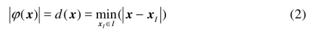
where I is the interface. It is not difficult to initialize the level set function to be the distance function, however, under the evolution of advection equation, it will not always remain in this way. Therefore, at later times in the computation, one must replace the level set function by a signed distance function without changing its zero-level set, which is called reinitialization. The straightforward method to reinitialize the level set function simply stands at each computational mesh point and finds the signed distance to the front. However, this can be time-consuming. Some efficient approaches are proposed to avoid explicitly finding the interface, such as solving an auxiliary advection-diffusion-like equation, or solving the Eikonal equation, etc..

The standard level set function (Eq.(2)) tracks all the level sets throughout the entire computational domain, which is not numerically efficient, because interest is actually confined only to the zero-level set itself corresponding to the interface. In order to decrease the computational labor, a narrow-band signed distance function is adopted, which is described in the following form:

where dsign=d( x), the sign is defined by Eq.(1) and d( x) is defined by Eq.(2), ε corresponds to half the thickness of the interface. On a discrete grid, the interface thickness is approximately equal to the characteristic grid size, so that the smooth profile can be resolved. As the grid elements increase, the interface thickness becomes thinner, and the control equations of two phase flow can be solved more accurately. However, under the evolution of advection and renormalization, the level set function will approximate the narrow-bound signed distance function.

2. Advection of the level set function

2.1 Advective step

The transport of the level set function φ over the domain Ω is generated by the velocity field v, and can be written as follows

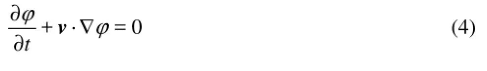
where the velocity field v is determined by solving the two-fluid N-S equations. In the water collapse case, there is no inflow or outflow existing, thus, the streamlines are closed all over the computational domain. At each time step, the level set function values are determined by the upstream ones, which are given values of the last time step in the same computational domain. So, there is no boundary condition required for the advection equation of the level set function. The initial condition is given by Eq.(3).

The numerical resolution of this advection problem is provided by FEM with some of the libraries of the PETSc-FEM code. Since the SUPG strategy is used in the Galerkin formulation when solving the transport of φ given by Eq.(4), the typical numerical instabilities can be eliminated.

2.2 Renormalization step

Within the pure advection procedure of the level set function, some requirements over the solution are not verified, such as keeping the transition strip with constant width. To solve this problem, Olsson et al.[16,17]proposed a renormalization equation after the advection step to keep the thickness and shape of the interface. Battaglia et al. proposed a similar renormalization equation, which is used in this work

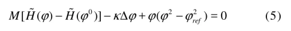
where M is the penalization coefficient, κ stands for the diffusion parameter, refφ is reference value for the variable φ, adopted as φref=1, and φ0represents the level set function initial value for the renormalization step provided by the advective step.

The penalizing term of Eq.(5), where the penalty coefficient M is used, allows to take into account the known values0φ, i.e., those determined in the advection stage. The aim of this term is to avoid the displacement of the interface, represented by the zero level set φ=0, by weighting Hˆ(φ)-Hˆ(φ0). In this term, the penalty coefficient M is positive and non-dimensional, and the value should be adopted as O(10nd+2), withdn the number of spatial dimensions involved. The penalizing function ˆ()Hφ is defined as the continuous expression

The argument of the function in Eq.(6) is chosen for concentrating the effect of the penalizing term nearby the interface.

The last two terms of the Eq.(5) form a stationary heat-conduction-like equation

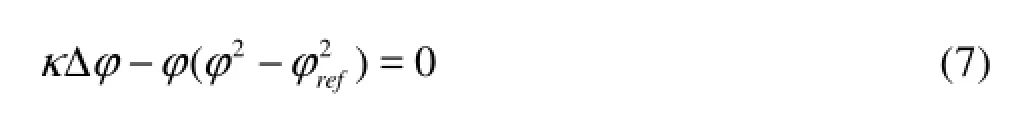
If the Laplacian term is neglected, i.e., =0κ, then the roots of the remaining heating source equation are φ=±φref=±1 and φ=0. In this situation, the level set function becomes a phase-field function with a discontinuous interface. In computations, the diffusion term (Laplacian term) is introduced to smear out the sharp interface, for achieving numerical robustness. It is verified that a larger value of the diffusion parameter lead to a wider transition of the interface. For the heat conduction equation, the same heating sources get the same temperature. In the same way, the same level set values get the same distance to the interface. So that, the converged result of the Eq.(7) will approximate the narrow-band signed distance function, and keep the interface thickness constant. The diffusion parameter κ is given in2lengh units, and is related to a typical mesh element size h, usually from2h to (3h)2, depending on the free surface behavior: a lower κ provides a thinner transition.

The regions placed far from the interface are not affected by the renormalization process because all the three terms in Eq.(5) tends to zero when φ≈φref. On the other hand, the higher influence of the operator is registered in the neighborhood of =0φ, where the loss of precision in the free surface position and mass loss is registered.

Regarding the selection of the free parameter values, κ and M, in cases where free surface would suffer breaking up or would fold several times it is convenient to adopt a low κ value and a high M one, because transitions should be thinner and M would avoid the disappearance of the drops.

3. Incompressible two phase flow

The fluid flow behavior of incompressible and immiscible two-fluid system is described by N-S equations in the following way:

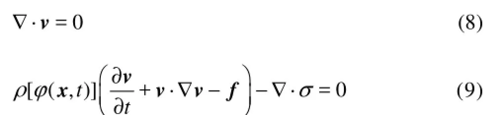
where Ω∈x is the position vector, v and f are the fluid velocity and body force, [(,)]tρ φx represents the fluid density, and φ is the level set function.

The fluid stress tensor σ can be determined as

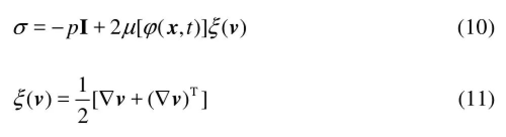
where p is the pressure, [(,)]tμ φx is the dynamic viscosity, I is the identity tensor, ()ξv is the strain rate tensor.

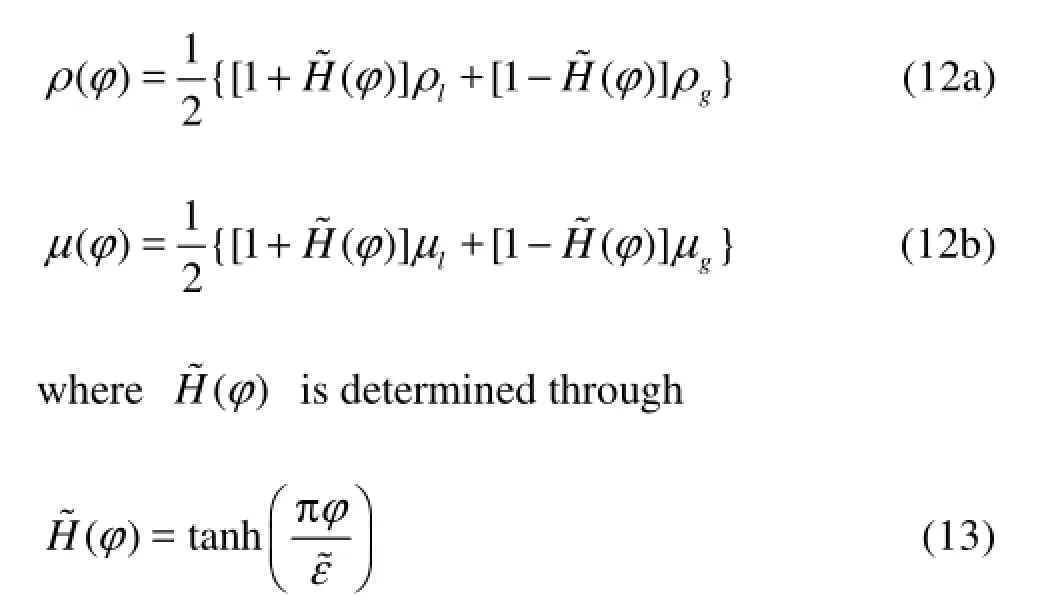
The level set function is defined by Eq.(1). Then, the fluid properties, density and dynamic viscosity, are given as functions of the φ values

For the water collapse with an obstacle case, boundary conditions for v in N-S equations are given over the solid boundarieswallΓ, and the pressure reference =0p is imposed at one point of the top domain.

The resolution is obtained through the N-S solver from the PETSc-FEM libraries, considering linear elements with the same interpolation for velocity and pressure fields, stabilized with SUPG and PSPG.

4. Results and discussion

Both 2-D and 3-D water collapse with an obstacle cases have been investigated numerically by many researchers using various methods. Greaves has simu-lated the same problem using adapting hierarchical grids with FVM-VOF method[18]. Zhang et al.[3]have studied the 3-D case by a modified MPS method, and so on. Experiment data have been provided by Koshizuka et al.[2]. In this work, both 2-D and 3-D water collapse with an obstacle cases are investigated.

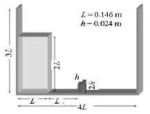
Fig.1 The sketch for water collapse problem

For 2-D case, the computational domain is 0.584 in length and 0.438 in height, the water column is defined by Wc=L=0.146 and Hc=2L=0.292 at t=0. The obstacle (0.024×0.048) is placed on the bottom of the tank, in the way of the moving front with its lower left corner in the centre of the tank. For 3-D case, the computational domain is 0.584×0.146×0.438, the initial statement of the water column is 0.146× 0.146×0.292, and the obstacle is 0.024×0.146×0.048. The geometry of computational model is given in Fig.1, and the initial statement is shown in Fig.3. At t=0, the velocity is zero everywhere. Then the restrain is removed instantaneously and the resulting collapse of the water column under gravity is simulated.

The fluid properties of water are chosen in the liquid phase and air in the gaseous one. The density is ρl=1000 and the dynamic viscosity is μl=1.0× 10-3for the liquid, and ρ=1, μ=1.0× 10-5for the gas.

The boundary conditions adopted for the fluid problem are perfect slip over the whole domain contour, which means 0·=v n, with n the vector normal to the contour, and the pressure reference =0p is imposed at one point of the top domain. The advection problem solved by the ADV module of PETSc-FEM does not require boundary conditions because there are not inflow sections in Ω.

The numerical simulation was performed up to a final time tf=0.6 in 300 time steps, with a time stepping of Δt =0.002and implicit temporal integration for the N-S and the ADV problems.

For 2-D case, the domain is discretized by 10 750 quadrangles. The typical element size is h≈0.00487. The parameters adopted for the renormalization are κ=4h2and M=10 000, at every time step. The computational mesh is shown in Fig.2(a).

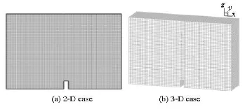
Fig.2 Computational mesh

For 3-D case, the domain is discretized by 40 275 hexahedrons. The typical element size is h≈0.00973. The renormalization parameters are κ=4h2and M =100 000. The computational mesh is shown in Fig.2(b).

Fig.3 The initial statement of water collapse with an obstacle

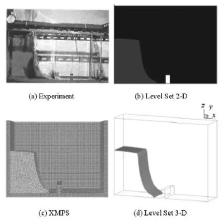
Fig.4 Results comparison (=0.1)t

The evolution of the free surface of the water collapse with an obstacle is shown from Fig.3 to Fig.8. The experiment images are presented by Koshizuka et al.[2], and the XMPS results are provided by Zhang et al.[3]. Generally, the level set results, including 2-D and 3-D case, keep reasonable agreement with the experiment image and the XMPS result. At =0.1t, thephotograph of experiment shows spray at the obstacle, indicating that the front tip has reached the obstacle. However, the predicted front tip, among all the numerical results, has not yet reached the obstacle. At =t 0.2, the movement of the front tip has been obstructed by the obstacle and a tongue of water bounces up from the upper left corner of the obstacle in the direction of the right-hand wall. At =0.3t, the predicted shape of the tongue of water is similar to that of the experiment as the tongue moves towards the right-hand wall. At t=0.4, the tongue impinges against the right-hand wall, trapping air beneath it. The sheet of water begins to fall under the action of gravity, but the trapped air provides resistance to this downward motion. However, the water of the XMPS result falls much quicker than the level set results, maybe due to its single phase model. At =0.5t, the sheet of water continues its downward motion. The trapped air resists the downward fall of the water. However, single phase XMPS model can not simulate this phenomenon at all. At the same time, a secondary tongue of water is generated at the obstacle and shoots into the trapped air space. However, the length of the tongue, predicted by the FEM-level set method, is shorter than the experimental one.

Fig.5 Results comparison (=0.2)t

Fig.6 Results comparison (=0.3)t

Fig.7 Results comparison (=0.4)t

Fig.8 Results comparison (=0.5)t

In Fig.9, the evolution of the free surface and the cut-plane of velocity vectors are presented. From the Figs.9(a) to 9(b), the water jet rushes along the bottom of the tank under the action of gravity. The velocity ofthe front tip becomes faster and faster. In Fig.9(c), the movement of the front tip has been obstructed by the obstacle, a tongue of water has been generated and moved upward. From the Figs.9(d) to 9(e), the collapsing water deflects the tongue to the right-hand wall. During this period, a primary eddy has been formed in the upper air space, and moved to the right-hand wall. In Fig.9(f), two water jets have been formed, one moves upward along the right-hand wall, and the other moves downward. At the same time, the sheet of water begins to fall under the action of gravity, but the trapped air resists this downward motion. In Fig.9(g), the downward water jet impinges the bottom wall, and moves to the left-side. In Fig.9(h), the sheet of water continues its downward motion. At the same time, a secondary tongue of water is generated at the obstacle and shoots into the trapped air space. The trapped air is pushed upward, and will eventually burst through the water sheet above it. In the whole evolution, the free surface and velocity field change violently. The level set results are demonstrated to reasonably capture all the details of flow observed in the experiment.

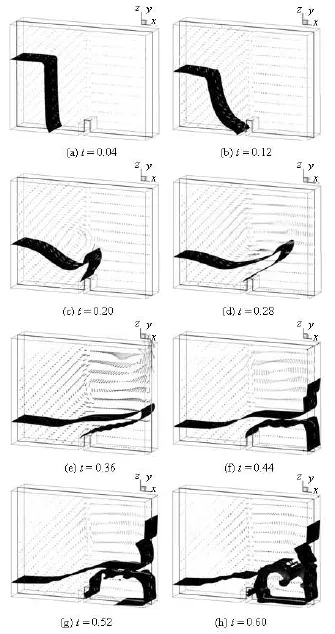
Fig.9 The evolution of the free surface and the cutplane of velocity vectors (level set 3-D)

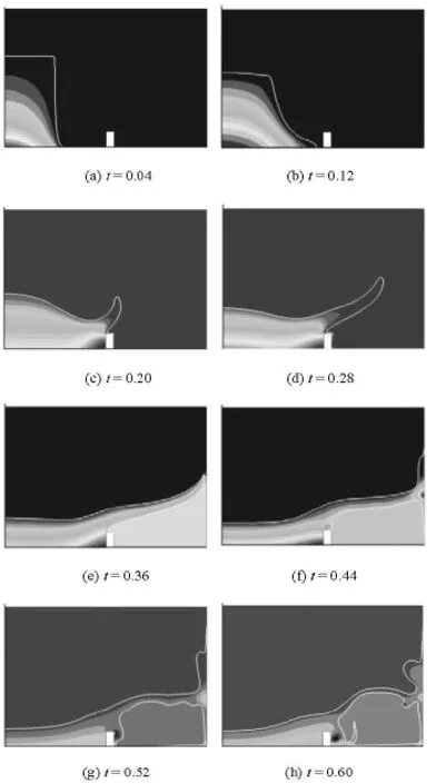
Fig.10 The evolution of the free surface and the pressure (level set 2-D)

The evolution of the free surface and pressure field are shown in Fig.10. In the Fig.10(c), the fast moving front tip has been obstructed by the obstacle, so the pressure becomes very large in a short time. In the Fig.10(e), the tongue of water impinges the righthand wall, trapping air beneath it. The sheet of water begins to fall under the action of gravity, so the pressure of the trapped air becomes larger and larger. In the Fig.10(f), when the tongue of water impinges the right-hand wall, the sudden surge of the pressure is due to the decrease of the kinetic energy.

5. Conclusions

An exhaustive implementation of the interfacecapturing approach based on a level set function to simulate transient two fluid viscous incompressible flows has been presented. Instead of the standard level set function, a narrow-band signed distance function is adopted to indicate the phase fields and the interface. Accordingly, a renormalization with continuous penalization procedure for the level set function is implemented to keep the thickness of the interface constant, which follows the advection procedure. By the level set function, a two-fluid N-S equation can be solved to capture the transient motion of free surface flow. Combined the finite element method with the level set method, the water collapse with an obstacle cases are simulated, both in 2-D and 3-D. The evolution of the free surface profile keeps good agreement with the experiment data and other numerical results. The evolution of the velocity vectors and pressure are also presented.

From these results, it is found that this FEM-level set method can simulate the 3-D water collapse with an obstacle efficiently and reasonably. In the next step, we will try to extend the numerical simulation to other free surface problems.

Acknowledgements

The authors are grateful to Battaglia Laura and Storti Mario A. for their help during using the code PETScFEM. High Technology of Marine Research Project of The Ministry of Industry and Information Technology of China and the Program for Professor of Special Appointment (Eastern Scholar) at Shanghai Institutions of Higher Learning (Grant No. 2013022), and center for High Performance Computing (HPC) at Shanghai Jiao Tong University for this work is gratefully acknowledged.

[1] WANG J., ZOU R. and WAN D. Numerical simulation of 3D dam-break flow by FEM-level set method[C]. The 22nd International Ocean and Polar Engineering Conference. Rhodes, Greece, 2012.

[2] KOSHIZUKA S., OKA Y. Moving-particle semi-implicit method for fragmentation of incompressible fluid[J]. Nuclear Science and Engineering, 1996, 123(3): 421-434.

[3] ZHANG Yu-xin, WAN De-cheng. Application of MPS in 3D dam breaking flows[J]. Scientia Sinica Physica, Mechanica and Astronomica, 2011, 41(2): 140-154(in Chinese).

[4] WANG J., WAN D. Numerical simulation of viscous flow with free surface around a structure using a moving mesh technique[C]. Proceedings of the Seventh International Workshop on Ship Hydrodynamics. Shanghai, China, 2011.

[5] SETHIAN J. A., SMEREKA P. Level set methods for fluid interfaces[J]. Annual Review of Fluid Mechanics, 2003, 35: 341-372.

[6] WAN De-cheng, SHEN Zhi-rong and MA Juan. Numerical simulations of viscous flows around surface ship by level set method[J]. Journal of Hydrodynamics, 2010, 22(5): 271-277.

[7] ZHAO Lan-hao, LI Tong-chun and NIU Zhi-wei et al. Fractional step FEM for calculation of 3D large amplitude sloshing problem using level set method[J]. Journal of Hydrodynamics, Ser. A, 2006, 21(4): 433-438(in Chinese).

[8] SUSSMAN M., PUCKETT E. G. A coupled level set and volume-of-fluid method for computing 3D and axisymmetric incompressible two-phase flows[J]. Journal of Computational Physics, 2000, 162(2): 301-337.

[9] ENRIGHT D., FEDKIW R. and FERZIGER J. et al. A hybrid particle level set method for improved interface capturing[J]. Journal of Computational Physics, 2002, 183(1): 83-116.

[10] GU Han-bin, LI Yan-bao and LI Shao-wu et al. The level set and particle level set method for tracing interface[J]. Journal of Hydrodynamics Ser. A, 2005, 20(2): 152-160(in Chinese).

[11] TUREK S., MIERKA O. and HYSING S. et al. A high order 3D FEM-level set approach for multiphase flows with application to monodisperse droplet generation[J]. International Journal for Numerical Methods in Fluids, 2010, 1-23.

[12] BATTAGLIA L., STORTI M. A. and ELIA J. D. An interface capturing approach with bounded continuous renormalization for free surface flows[J]. Mechanical Computation, 2009, 28(1): 1423-1440.

[13] BATTAGLIA L., STORTI M. A. and ELIA J. D. Bounded renormalization with continuous penalization for level set interface-capturing methods[J]. International Journal for Numerical Methods in Engineering, 2010, 84(7): 830-848.

[14] SONZOGNI V. E., YOMMI A. M. and NIGRO N. M. et al. A parallel finite element program on a Beowulf cluster[J]. Advances In Engineering Software, 2002, 33(7-10): 427-443.

[15] PAZ R. R., NIGRO N. M. and STORTI M. A. On the efficiency and quality of numerical solutions in CFD problems using the interface strip preconditioner for domain decomposition methods[J]. International Journal for Numerical Methods in Fluids, 2006, 52(1): 89-118.

[16] OLSSON E., KREISS G. A conservative level set method for two phase flow II[J]. Journal of Computational Physics, 2005, 210(1): 225-246.

[17] OLSSON E., KREISS G. and ZAHEDI S. A conservative level set method for two phase flow[J]. Journal of Computational Physics, 2007, 225(1): 785-807.

[18] GREAVES D. M. Simulation of viscous water column collapse using adapting hierarchical grids[J]. International Journal for Numerical Methods in Fluids, 2006, 50(6): 693-711.

10.1016/S1001-6058(15)60463-2

* Project supported by the National Natural Science Foundation of China (Grant Nos. 51379125, 51411130131 and 11432009), The National Key Basic Research Development Program of China (973 Program, Grant No. 2013CB036103).

Biography: WANG Ji-fei (1984-), Male, Ph. D.

WAN De-cheng, E-mail: dcwan@sjtu.edu.cn