ZHANG Xue-lan （张雪兰）, SUN Xi-huan （孙西欢）,2, LI Yong-ye （李永业）

1. College of Water Resource and Engineering, Taiyuan University of Technology, Taiyuan 030024, China, E-mail: hbxiehou@126.com

2. Shanxi Conservancy Technical College, Yuncheng 044004, China

3-D numerical investigation of the wall-bounded co*ncentric annulus flow around a cylindrical body with a special array of cylinders

ZHANG Xue-lan （张雪兰）1, SUN Xi-huan （孙西欢）1,2, LI Yong-ye （李永业）1

1. College of Water Resource and Engineering, Taiyuan University of Technology, Taiyuan 030024, China, E-mail: hbxiehou@126.com

2. Shanxi Conservancy Technical College, Yuncheng 044004, China

(Received March 31, 2014, Revised June 3, 2014)

Concentric annulus flow around a combinational cylindrical body with a special array of cylinders at five high Reynolds numbers is investigated numerically using Fluent 6.3.26 in this paper. The numerical results show a good agreement with the experimental data in regard to the axial velocity of the flow. This study focuses on the flow structure and the hydrodynamic characteristics based on the velocity distribution, the pressure distribution, streamlines and vectors under 1-D, 2-D and 3-D conditions. Meanwhile, some global parameters including the pressure coefficient, the drag coefficient and the lift coefficient are analyzed. Numerical results show that the high velocity region and the reverse wake zone with low velocity exist in some spaces due to the disturbance of the cylindrical body. Negative pressures appear in some regions. Neither a wide area vortex nor the vortex shedding appears in the wall-bounded domain. The drag along the axial direction is the main force acting on the cylindrical body in the pipe domain. The annulus flow around the cylindrical body is analyzed to reveal the hydrodynamic characteristics of the complex turbulent concentric annulus flow field due to the multi-effects in the pipeline.

numerical simulation, concentric annulus, high Reynolds number, cylindrical body, hydrodynamic characteristics

Introduction

The flow around multiple cylinders has been a research focus for a long time, with considerations of different influencing factors, including the shape, the number and the arrangement of cylinders, the Reynolds number and the computational domain boundary. Numerical investigations play an important role. When the fluid flows by multiple cylinders in a special array, the dynamic features will vary much more than while passing a single one due to the interference effects[1,2]. Zdravkovich[3]illustrated that the interference depends on the relative positions of two cylinders and their locations in the free stream to a certain degree. In the investigation, three arrangements were discussed: the staggered, the tandem and the side-by-side ones. Zhang et al.[4]performed a 2-D study to model two cylinders with different diameters using Fluent. Two flow models in the cavity flow pattern and the wake impinge flow pattern would appear with the variation of the spacing between the two cylinders. Chattejee et al.[5]performed a numerical study of the flow around five square cylinders with two arrangements at a low Reynolds number to reveal three flow patterns: the in-phase and antiphase synchronized model, the flip-flopping model and the non-synchronized model. Bao et al.[6]numerically investigated the flow around seven square cylinders in an inline array with different spacing ratios. It was concluded that a critical value of the spacing ratio exists in the flow pattern transition from steady to unsteady states. Kumar et al.[1]increased the number of square cylinders up to nine and decreased the Reynolds number level. Flow regimes, including chaotic, quasi-periodic and synchronize ones, were indentified through the numerical study. Huang et al.[7]assumed an incompressible flow in their 2-D simulations to study the waterflow over two rows of cylinders in staggered array showing the formation of Kaman vortices between two cylinders rows.

Besides, the Reynolds number and the boundary at a small calculation region are another two influencing factors. In previous studies, the Reynolds numbers varied from low to high in the range of 100≤ Re≤500[8-10]and up to the range of 1.4× 105≤Re ≤ 5× 106[11,12]. These studies show that the Reynolds number is a critical influencing parameter for the aerodynamic characteristics such as the force coefficients, the Strouhal number, the pressure distribution and so on. Many investigations indicated that the flow boundary characteristics contribute significant impacts on the development of the flow field[13-15]. In the limited calculation region, the wall-bounded flow has different flow features than the free stream due to the interference from boundaries[16,17]. Under conditions smooth enough with high Reynolds numbers, the wall-bounded flow may stay at a laminar state and a discontinuous transition to turbulence appears after sharp perturbations, which is different from the bulk shear flow, which becomes turbulent at low Reynolds numbers[18]. Recent studies show that the transitional regime in a fixed computational domain of a pipeline with a limited diameter contains chaotic puffs which would become turbulent slugs as the Reynolds number increases[19].

In the present investigation, a defined cylindrical body is placed in a horizontal pipe to form a concentric annulus space. The flow around the body becomes turbulent due to the sudden disturbance. Some improvements are made on the previous investigations. Firstly, the cylindrical body structure consists of a main cylinder with a larger diameter and six small attaching cylinders of equal sizes, which are arranged on the two end faces of the main cylinder in a radial distribution. Secondly, these cylinders used in the body and the pipe diameter are finite to form a limited calculation domain. Thirdly, the axes of the main cylinder and the pipe are coincident, to enable a comparison with the free cross flow around cylinders. Based on the above description, a further analysis on the characteristics of the flow is a critical step to discuss the flow structure and the pipe maintenance.

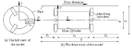
Fig.1 Schematic diagrams of the calculated geometry of the model and parameters

1. Geometry model

To study the flow around cylinders in a limited domain and relate the flow with the pipe flow, a cylindrical body structure is designed to form a concentric annulus flow in a horizontal pipe. The structure of the defined cylindrical body with a special cylinders array is shown in Fig.1(a) and the calculated parameters of the model are illustrated in Fig.1(b). As shown in Fig.1(a), the geometry model of the cylindrical body mainly contains two parts: the main cylinder with diameter d and six attaching cylinders with diameter /6d. These attaching cylinders are arranged on the two end faces of the main cylinder in a radial distribution. The interval angle between two neighboring attaching cylinders iso120. The connecting component between the two parts is a small sheet. The length of the main cylinder is L1/d=5/3 and the attaching cylinder is L2/d=1/2. The cylindrical body is located in the straight pipe, whose inner diameter is D/ d=5/3, with a zero vertical angle. One end of each attaching cylinder is supported on the pipe wall to make the axes of the pipe and the main cylinder to be coincident. Thus, a concentric annulus space around the main cylinder is formed. Then, the flow field formed by the cylinders array is named as the concentric annulus flow field. The end of the attaching cylinders, which is supported on the pipe wall, is a semi-sphere of the diameter equal to that of the attaching cylinders. A Cartesian coordinate is established and the coordinate origin is located at the center of the upwind end of the main cylinder and the positive direction of -Zaxis is along the coming flow direction.

2. Governing equations, numerical details and validation study

The numerical simulation is a part of a series of investigations of the concentric annulus turbulent flow,which include numerical studies and experimental studies with fixed test conditions. For the consistency of these investigations, five Reynolds numbers (denoted as Re1=76 738, Re2=102317, Re3=127896, Re4=153476, Re5=179 055) are assumed in the simulation according to the parameters in the experiments. The order of magnitude of the five investigated Reynolds numbers is at a high level, therefore, the assumption of the turbulence flow is valid. The 3-D numerical simulation of the unsteady incompressible fluid flow is performed under the initial condition of the mean velocity in the inlet. And the fluid in the simulation is a liquid of constant viscosity and density. Breuer et al.[20]indicated that the numerical calculations at higher Reynolds numbers need higher resolutions. Comparing with other calculation models for high Reynolds number, the standard -kε model is the most widely used one with a relatively low demand for the CPU memory and the computational speed. And also, fewer differential equations are involved than the RSM and the workload is reduced. The standard -kε model is adopted for an efficient numerical simulation. The governing equations are:

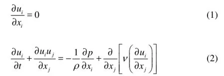
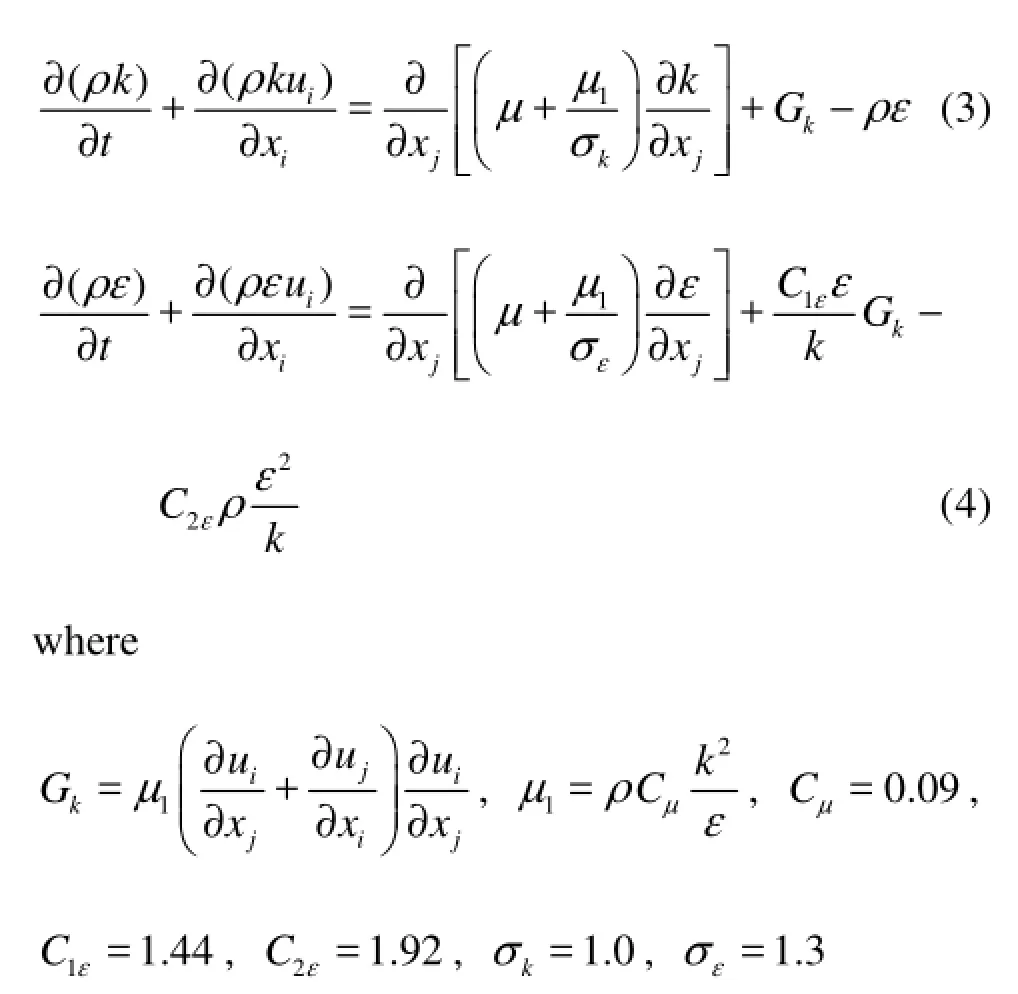
where ν is the kinematic viscosity, and ρ is the density of the fluid. In the standard -kε model, the transport equations corresponding to the two unknown parameters (k and ε) are

SIMPLEC scheme with the second order accuracy in Fluent 6.3.26 is used in the simulation. The calculated domain s includes the length1s from the inlet to the upwind end of the cylindrical body, the length2s from the outlet to the downwind end and the length of the body. The inlet boundary 10d away from the upwind end of the cylindrical body is specified as the velocity inlet boundary with0=vv. Owing to the different Reynolds numbers, the value of0v is reset correspondingly in the simulation under a changed Reynolds value. The outlet 20d away from the downwind end of the cylindrical model is set as the “pressure-outlet”. In the inlet boundary, the turbulent kinetic energyink and the turbulent dissipation rateinε are given as

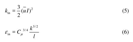
where the intermediate computations of the turbulence intensity involve I=0.16(ReD)-1/8(where ReDis the Reynolds number computed by the hydraulic diameter), and the turbulence length scale is =0.07lD. Both the investigated walls of the pipe and the cylinders are made of plexiglass. Thus, the roughness heightsK under the wall boundary condition is set to be 10–5m and the roughness constantkC is 0.5. In the grid system, a boundary layer is established by denser clustering of the mesh points near the pipe wall. The boundary layer is fixed as four rows with the first row of 0.005 and the growth factor of 1.2. Outside the boundary layer, the volume grid with an interval size of 0.5 is used to balance the accuracy and the efficiency of the calculation. The grid system is created reasonably with+y being adjusted suitably for the wall treatment selected, where the number of the iterating time steps is 500 with a step size of 0.005. In these iteration processes for five Reynolds numbers, all simulations are converged, with the residuals in all equations less than 0.001, and the flow develops fully with enough data for the statistical analysis.

In the investigation, the flow pattern, the pressure distribution and some global parameters are analyzed. The lift coefficient (Cl), the drag coefficient (Cd) and the pressure coefficient (Cp) are defined as follows

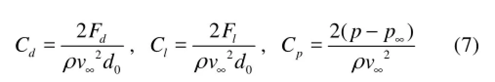
wheredF andlF are the drag force in the pipe stream direction and the lift force in the vertical direction, respectively, p∞, v∞and0d are the characteristic pressure, velocity and diameter, respectively.

Fig.2 Comparison between numerical and experimental -Zdirection velocities

The agreement of the numerical results with the experimental data by comparing the -Z direction velocity in two representative cross sections at the Reynolds number3Re is shown for the example in Fig.2. The first selected section z/ s=0.345 (see Fig.2(a), z is the coordinate value along -Z axis), where /z s stands for the section location and its starting point is located at the inlet, is in the annulus space around the main cylinder. The other section /z s=0.288 is in front of the cylindrical body (see Fig.2(b)). The -Z direction velocities at several sample points are compared in each figure. According to the symmetry with -Xaxis as the symmetry axis in these sections, only the sample points located on one half part (/0y D≥, y is the Y coordinate value of a point) are selected. It is shown in the two figures that some small differences exist between the numerical data and the experimental data. The possible cause of the differences is that in the standard -kε model, a certain distortion will occur in the flow simulation with the bending boundary due to the assumption of the isotropic viscosity coefficient referring to each component of the Reynolds stress. However, the agreement is considered to be good enough as seen from the same trends and very small differences. Thus, the numerical calculation can be carried out to investigate the complex annulus flow field.

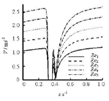
Fig.3 Velocity distribution along -Zaxis for each Reynolds number

3. Results and discussions

3.1 Velocity characteristics

The sectional mean velocity along -Zaxis is shown in Fig.3 for each Reynolds number. In these curves, a segment of the flow velocity is missing in the range from /=z s0.318 to 0.371 due to the presence of the main solid cylinder on the axis. For all Reynolds numbers, the velocity distributions along z/ s see a same trend. Sharp decreases in front of the main cylinder and “N”-shaped fluctuations behind it occur, which implies that the obstruction of the cylindrical body leads to low velocity zones. But the range of the following low velocity zone is larger than the front velocity decreasing zone. In regions far away from the cylindrical body, the velocity value rises up gently.

For clear illustrations of the flow features around the cylindrical body, some local segments of the calculated domain are shown in Fig.4. From the 2-D velocity contours, it can be seen that low velocity zones are shaped as a tongue behind the cylindrical body both in Section /=0x D (Fig.4(a)) and Section /y D=0 (Fig.4(b)). An oval region with higher velocity than that in its surrounding area occurs in the tongueshaped zone, which is consistent with the velocity curve shaped like “N” in Fig.3. Besides, two obvious high velocity zones exist in the space above and below the main cylinder in Section /=0x D owing to the reduced overflow area. In Section /=0y D, two high velocity zones are unsymmetrically distributed as a result of the disturbance from attaching cylinders. Except for the left high velocity zone between two attaching cylinders in Section /=0y D, other high and low velocity zones gradually disappear with thespread downstream. For further explorations of the special high velocity zone in Section /=0y D, the velocity contours in Section x/ D=0.4 (Fig.4(c)) are shown. In Fig.4(c), a fishtail-shaped high velocity zone is seen. The following attaching cylinder separates the zone into two parts in its rear. Thus, it appears that the left high velocity zone just stays between the two attaching cylinders without spreading downstream in Fig.4(b). Figure 4(d) illustrates the vector distribution of the velocity in Section /=0x D. It is shown that the velocity vector direction, initially along -Z axis of the pipe, is changed to transit into the annulus at the upwind side of the main cylinder. And a pair of symmetry reverse regions appears in the tongue-shaped low velocity zone behind the main cylinder. Unlike what shown in Fig.4(d), there is not a reversing wake generated after any attaching cylinder in Fig.4(e), in which the streamlines are around a pair of attaching cylinders. Fig.4(d) shows that outside the reverse regions, the vector direction returns to be parallel to -Z axis. And in Fig.4(e), after passing each attaching cylinders, streamlines are parallel forward. The former phenomenon in the two figures is due to the fact that the flow makes a redistribution in a very short time after the sudden disturbance in the long pipe with a small diameter.

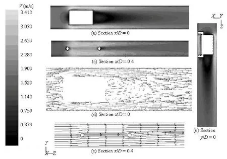
Fig.4 Velocity contours, vector and streamline maps in several longitudinal sections at the Reynolds number3Re

In order to study the velocity distributions along X-axis and Y-axis, several feature cross sections are selected along the Z- axis direction. Among these sections, the range of 0≤z/ s ≤0.136 is in front of the main cylinder, 0.319≤z/ s ≤0.370 is in the annulus space. The velocity distributions along the directions of -Xaxis and -Yaxis in these spaces are shown in Fig.5.

In the segment in front of the cylindrical body, the velocity distribution in Section /=0z s is flat due to the velocity inlet boundary (see Fig.5(a)). As the fluid flows forward, the velocity follows a logarithmic law, which is consistent with the suggested turbulent velocity distribution in the pipe as indicated in Hydraulics textbooks. This is the evidence that the set of s1is long enough for the pipe flow full development before the sudden disturbance. The same situation appears in the downstream far away from the cylindrical body. In the sections near the cylindrical body, the velocity in regions near /=0x D and /=0y D goes down and the velocity in their surrounding areas rises up. The presence of the attaching cylinders leads to zero velocity regions at 0.2≤x/ D ＜0.5 as shown in Fig.5(a). And, the sharp increase of the velocity in front of the cylindrical body occurs in the small gap between the hemispherical end of the attaching cylinder and the pipe wall. Unlike the velocity along /x D, that along /y D shows a symmetrical distribution at the two sides of /=0y D. The symmetry along y/ D also exists in the annulus space and behind the main cylinder. In the annulus space around the main cylinder (Fig.5(b)), “n”-typed curves with higher velocity peaks appear as the result of the shrunken overflow area, which confirms the high velocity zone analysis in Figs.4(a) and 4(b). The zero velocity zones are produced by the main cylinder. In all figures in Fig.5, sudden decreases of the velocity are observed near the walls of the pipe and the cylindrical body owing to the boundary viscous effect.

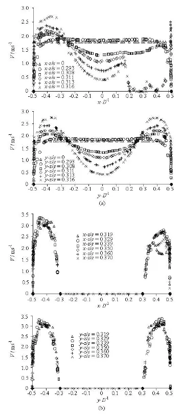
Fig.5 Velocity distributions along X-direction and Y-direction in feature cross sections at the Reynolds number Re3

In the analysis of flow in the downstream space behind the main cylinder, a general similar situation exists in the velocity distribution in sections behind the cylinder. But, unlike the velocity in the disturbed space in front of the cylindrical body, a slight velocity rise near /=0x D or /=0y D occurs in the low velocity region behind the body, which is consistent with the oval higher velocity regions shown in Figs.4(a) and 4(b). At the outlet, the same logarithmic distribution as at the inlet implies that the set of2s is suitable for the flow to fully spread after the sudden disturbance.

Fig.6 Distribution curves of sectional mean pressure along -Z axis

3.2 Pressure characteristics

The distributions of the mean pressure in the cross sections along -Z axis for all Reynolds numbers are presented in Fig.6. Due to the obstacle body, a segment of /z s is missing in the figure. It is shown that the mean pressure goes down slowly in large regions in front of and behind the cylindrical body due to the water head loss. Near the upwind end of the cylindrical body is a small region of the pressure lifting owing to the decreasing velocity. And in the nearby region behind the main cylinder, the pressure goes up sharply after a slight decrease, which is because of the velocity variation in the tongue-shaped low velocity zone. It is known from Fig.6 that the higher Reynolds number tend to raise the pressure without changing the distribution trend in front of the cylindrical body, to increase the peak value and decrease the lowest value behind the cylindrical body. The -Z axis end at the outlet is the zero pressure point because of the“pressure-outlet” setting.

Fig.7 Distribution of sectional mean pressure coefficient in -Z direction

Fig.8 Circumferential pressure distributions on surfaces of the main cylinder and the attaching cylinders at the Reynolds number3Re

Figure 7 illustrates the distribution of the sectional mean pressure coefficient in -Z direction for each Reynolds number. In the distribution for each Reynolds number, a sharp decrease and increase is seen near the two ends of the cylindrical body. In the annulus range, an “n”-shaped distribution appears with the lowest values located there. In the other places far away from the cylindrical body,pC decreases slowly along /z s. The pressure coefficients are zero at the pipe outlet due to the “pressure-outlet” boundary setting. Except for the outlet, it can be seen from Fig.7 that a higher Re value leads to a lower pressure coefficient with small differences.

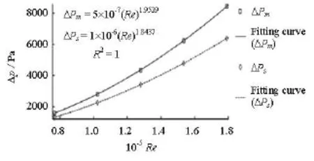
Fig.9 Fitting curves of pressure drop

Figure 8(a) shows the circumferential pressure distributions at z/ s=0.319 (annulus upwind end), z/ s=0.345 (middle location in annulus) and z/ s= 0.370 (annulus upwind end) on the main cylinder surface from the starting point of “0” in the clockwise direction. Figure 8(b) shows the circumferential pressure distribution at x/ D=0.4 on the surfaces of attaching cylinders located on the upwind end and the downwind end of the main cylinder. Starting point of“0” in a Cartesian coordinate is marked in each figure and the positive direction of the third axis in each coordinate is pointing normal to the paper downward. Due to the symmetry, the angle range ofoo0-180 is analyzed. It is observed in Fig.8(a) that the negative pressure surrounds the longitudinal surface of the main cylinder, which may lead to cavitation erosion. Among the three curves at different /z s, the curve at z/ s=0.319 fluctuates violently principally caused by the integrated interference of the sudden changes of the flow at the annulus upwind end and the transmitted disturbance of the attaching cylinders. In the following position, the flow field develops for a short time in the annulus to produce a more smooth pressure distribution. At z/ s=0.370, an integrated action from the downwind end of the annulus and the attaching cylinders there is added, whose disturbance to the flow in front of them is weaker than that behind. Thus, a small fluctuation difference occurs on the pressure curves there as compared with that at the position z/ s=0.345. In Fig.8(b), the pressure on the surface of the downwind attaching cylinder, where a negative pressure appears, is lower than that upwind due to the water head loss. From the two curves, it is seen that the pressure generally stays in three different levels owing to the variety of the nearby velocity along the stream direction around a cylinder. On the downwind attaching cylinder surface, the conspicuous points with a lower pressure than that at the neighboring points are in the second pressure segment (angle of 70o-110o) because of the downstream propagationproduced by the annulus high velocity, which is different from the upwind attaching cylinder.

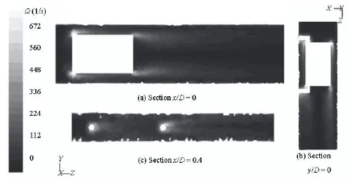
Fig.10 Vorticity contours at several feature sections at the Reynolds number3Re

Fig.11 3-D streamline and velocity vector maps at the Reynolds number3Re

The pressure drop between positions z/ s= 0.308 and z/ s=0.381 (denoted as ΔPm), which is mainly caused by the local water head loss due to the cylindrical body, and the pressure drops of the total pipeline (denoted assPΔ) are fitted in Fig.9. It is shown that good power law relationships exist between the pressure drop and the Reynolds number. Obviously, the variation magnitude ofmPΔ with Re is higher than that ofsPΔ. And formulas representing the relationships are marked in the figure. Thus, the pressure drop for any Reynolds number in the range of 15-ReRe can be estimated easily using these formulas.

3.3 Vorticity characteristics

The vorticity contours at Section /=0x D (Fig.10(a)) and /=0y D (Fig.10(b)) show that the edges of the two ends of the main cylinder produce a weak vortex, which disappears without shedding in a short region in the downstream. In the pane of /=x D 0.4 (Fig.10(c)), there are steady vortex zones without shedding around the attaching cylinders. But these zones are small due to the small size of these cylinders and the superimposed effect from the annulus flow. From the above analysis, it is concluded that no wide range vortex is produced by the cylindrical body in the limited wall-bounded domain.

3.4 3-D flow features

This section discusses the distributions of dynamic parameters in the global domain for further investigation on the flow features. Figure 11 show the 3-D charts of the streamline around the cylindrical body, which reveals the characteristics. From the streamline pattern around the main cylinder (Fig.11(a)), it can be seen that the streamlines both in the annulus and far from the cylindrical body ends are parallel to the pipe axis. The streamline spacing is narrowed while reaching the upwind end of the main cylinder and is expanded out of the annulus with a pair of reverse wake zones next to the downwind end of the main cylinder. The streamlines around a pair of attaching cylinders are shown in Fig.11(b), which explains that the streamlines far away from the side surface of the main cylinder just pass the attaching cylinders without a reverse wake behind any one and the streamlines next tothe surface are in a reverse direction in the wake zone of the main cylinder. The velocity vectors appear parallel to the pipe axis at the pipe outlet (see Fig.11(c)), which implies that no back flow occurs there. The 3-D streamline appearance provides an intuitive display about the flow pattern for an easy understanding.

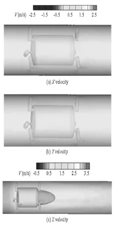
Fig.12 3-D velocity distributions in three directions at the Reynolds number3Re

Figures 12(a) and 12(b) show the 3-D distributions of the velocities in -Xdirection and -Ydirection around the cylindrical body. It is observed that the obvious nonzero velocity at the two directions only exists in some local small regions near the two ends of the main cylinder and the surfaces of the attaching cylinders and the connecting sheet, where the velocity vector changes its direction due to the obstacle to redistribute the velocity values in three dimensions. In other spaces of the investigated domain, the velocity value in the two directions is about zero because the velocity parallel to -Z axis is in the main stream direction of a slender pipeline. For the -Z direction velocity (Fig.12(c)), the velocity value decreases gradually while reaching the cylindrical body and a bulletshaped wake zone appears behind the cylindrical body, which is consistent with the tongue-shaped low velocity zone in the 2-D shows. The -Z direction velocity turns to be higher in the internal area of the pipe and lower near the wall. Besides, the apparent higher velocity surrounding the body is due to the sudden contraction of the overflow area. It is concluded that the Z velocity shows a general similar distribution as the aggregate velocity of the wall-bounded annulus flow in a slender straight pipe.

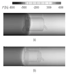
Fig.13 3-D pressure distributions at the Reynolds number3Re

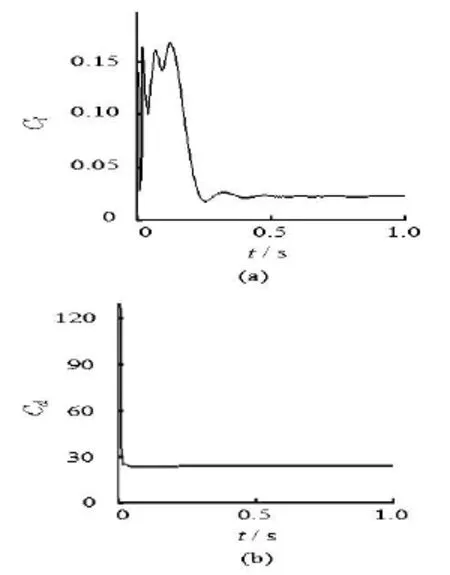
Fig.14 Monitoring curves of force coefficients of the cylindrical body at the Reynolds number3Re

Figure 13 shows the 3-D pressure distribution at a segment containing the cylindrical body. The upwind face of the cylindrical body is the conspicuous critical interface of the pressure declining along the flow direction. Figure 13(a) shows the pressure in a front view along the flow direction and Fig.13(b) is in the back in the reverse direction of the stream. The upwind end of the main cylinder is an apparent higher pressure face as compared with the surrounding pre-ssure, because of the zero velocity there. But the downwind end is not a differentiated pressure face compared with its surrounding pressure. In the annulus, the pressure drops to be negative and gradually increases to be positive after passing the body. A small region with the lowest negative value is in the place between the end of the attaching cylinder on the downwind end and the pipe wall. The serious cavitation erosion, which is adverse for the aegis of the pipe and the cylinder, might be the cause of the small region. In summary, the 3-D maps of the flow have a good consistency with the 1-D and 2-D analyses and provide a more intuitive picture about the flow features.

3.5 Force statistics

In the present investigation, the drag force is in the positive direction of -Z axis and the lift force is along the positive -Ydirection. The monitoring curves of the drag coefficient and the lift coefficient of the cylindrical body are shown in Fig.14. From the figure, it is observed that the two force coefficients become steady in a short calculation time with the lift coefficient fluctuating weakly in the first one tenth flow time.

These force coefficients on each part of the cylindrical body for each Reynolds number are given in Table 1. In the table, the drag coefficients of all investigated objects decrease with the increase of the Reynolds number and the lift coefficients take the lowest values at the Reynolds number2Re. The drag coefficient of the main cylinder is 3.6-3.7 times of that of the attaching cylinders, but the lift coefficient is much smaller with a difference of two orders of magnitude. The lift coefficient of the cylindrical body is negative so that the lift force on the body is along the negative -Ydirection. From the table it is seen that the force in -Z direction is the main force affecting the cylindrical body because the order of magnitude of the drag coefficient is much larger than that of the lift coefficient.

Table1 Force coefficients of the cylindrical body at each Reynolds number

4. Conclusions

In this study, a cylindrical body with an array of cylinders of a different size is located in the horizontal pipe to form a wall-bounded flow in the concentric annulus, as a new improvement of the flow around cylinders and a supplement to the pipe turbulent flow researches. The annulus flow characteristics due to the cylindrical body with the special cylinders array and the effect of the Reynolds number on the flow features are studied numerically using Fluent 6.3.26. Numerical results of the pipe axial velocity are compared with the experimental results. An acceptable agreement implies that the numerical simulation is valid. 3-D simulations for five Reynolds numbers are carried out. Some main findings are as follows:

(1) An “N”-shaped low velocity zone, a tongueshaped reverse wake zone in the sectional contour maps, exists behind the main cylinder on -Z axis and a sharp decrease occurs in front of the cylindrical body. Due to the viscosity on wall boundaries of the pipe and the cylindrical body, regions with sharply declining velocity are formed nearby. Increased Reynolds number increases the velocity value without changing the distribution trend. The annulus space is a high velocity zone.

(2) A higher Reynolds number leads to a lower sectional mean pressure coefficient along the pipe. Negative pressure exists in some local spaces of the pipe, which may lead to cavitation erosion. Neither wide range vortex nor vortex shedding due to the cylindrical body occurs in the pipe.

(3) The 3-D streamline and vector maps can visualize the flow pattern around the cylindrical body and the distributions of the velocity and the pressure in three dimensions show the flow features.

(4) Unlike the lift coefficient, the drag coefficient decreases with the increase of the Reynolds number. The values of the two force coefficients differ by two orders of magnitude, which means the drag along -Z direction is the main force on the cylindrical body inthe pipe domain.

These results help to understand the hydrodynamic characteristics of the integrated flow due to the complex cylindrical body and the pipe wall. In the future work, the number of the cylindrical bodies should be increased to study better the flow structure.

[1] KUMAR S. R., SHARMA A. and AGRAWAL A. Simulation of flow around a row of square cylinders[J]. Journal of Fluid Mechanics, 2008, 606: 369-397.

[2] ZOU Lin, GUO Cong-bo and XIONG Can. Flow characteristics of the two tandem wavy cylinders and drag reduction phenomenon[J]. Journal of Hydrodynamics, 2013, 25(5): 737-746.

[3] ZDRAVKOVICH M. Flow around circular cylinders, Vol. 2: Applications[M]. New York, USA: Oxford University Press, 2003.

[4] ZHANG P., WANG J. and HUANG L. Numerical simulation of flow around cylinder with an upstream rod in tandem at low Reynolds numbers[J]. Applied Ocean Research, 2006, 28(3):183-92.

[5] CHATTERJEE D., BISWAS G. A. and MIROUDINE S. Numerical simulation of flow past row of square cylinders for various separation ratios[J]. Computers and Fluids, 2010, 39(1): 49-59.

[6] BAO Y., WU Q. and ZHOU D. Numerical investigation of flow around an inline square cylinder array with different spacing ratios[J]. Computers and Fluids, 2012, 55: 118-131.

[7] HUANG Z., OLSON J. A. and KEREKES R. J. et al. Numerical simulation of the flow around rows of cylinders[J]. Computers and fluids, 2006, 35(5): 485-491.

[8] SHARMAN B., LIEN F. S. and DAVIDSON L. et al. Numerical predictions of low Reynolds number flows over two tandem circular cylinders[J]. International Journal for Numerical Methods in Fluids, 2005, 47(5): 423-447.

[9] SAHA A. K., BISWAS G. and MURALIDHAR K. Three dimensional study of flow past a square cylinder at low Reynolds numbers[J]. International Journal of Heat and Fluid Flow, 2003, 24(1): 54-66.

[10] ZHAO M., CHENG L. and TENG B. et al. Numerical simulation of viscous flow past two circular cylinders of different diameters[J]. Applied Ocean Research, 2005, 27(1): 39-55.

[11] MICHAEL B. A challenging test case for large eddy simulation: High Reynolds number circular cylinder flow[J]. International Journal of Heat and Fluid Flow, 2000, 21(5): 648-654.

[12] PIETRO C., WANG M. and GIANLUCA I. et al. Numerical simulation of the flow around a circular cylinder at high Reynolds numbers[J]. International Journal of Heat and Fluid Flow, 2003, 24(4): 463-469.

[13] COTTET G.-H., PONCET P. Advances in direct numerical simulations of 3D wall-bounded flows by vortexin-cell methods[J]. Journal of Computational Physics, 2004, 193(1): 136-58.

[14] FUREBY C., GRINSTEIN F. F. Large eddy simulation of high-Reynolds-number free and wall-bounded flows[J]. Journal of Computational Physics, 2002, 181(1): 68-97.

[15] HARICHANDAN A. B., ROY A. Numerical investigation of flow past single and tandem cylindrical bodies in the vicinity of a plane wall[J]. Journal of Fluids and Structures, 2012, 33: 19-43.

[16] FEDOSOV D. A., PIVKIN I. V. and KARNIADAKIS G. E. Velocity limit in DPD simulations of wall-bounded flows[J]. Journal of Computational Physics, 2008, 227(4): 2540-59.

[17] PRABHU R., COLLIS S. S. and CHANG Y. The influence of control on proper orthogonal decomposition of wall-bounded turbulent flows[J]. Physics of Fluids, 2001, 13(2): 520-37.

[18] MANNEVILLE P. Turbulent patterns in wall-bounded flows: A turing instability?[J]. Europhysics Letters, 2012, 98(6): 64001.

[19] AVILA K., MOXEY D. and De LOZAR A. et al. The onset of turbulence in pipe flow[J]. Science, 2011, 333(6039): 192-196.

[20] BREUER M., BERNSDORF J. and ZEISER T. et al. Accurate computations of the laminar flow past a square cylinder based on two different methods: lattice-Boltzmann and finite-volume[J]. International Journal of Heat and Fluid Flow, 2000, 21(2): 186-196.

10.1016/S1001-6058(15)60464-4

* Project supported by the National Natural Science Foundation of China (Grant Nos. 51179116, 51109155).

Biography: ZHANG Xue-lan (1986-), Female, Ph. D. Candidate

SUN Xi-huan, E-mail: sunxihuan@tyut.edu.cn