Li Yuanjin Shu Huazhong Luo Limin Chen Yang Wang Tao Yue Zuogang

(1Laboratory of Image Science and Technology, Southeast University, Nanjing 210096, China)(2School of Computer and Information Engineering, Chuzhou University, Chuzhou 239000, China)



Application of the Delaunay triangulation interpolationin distortion XRII image

Li Yuanjin1, 2Shu Huazhong1Luo Limin1Chen Yang1Wang Tao2Yue Zuogang2

(1Laboratory of Image Science and Technology, Southeast University, Nanjing 210096, China)(2School of Computer and Information Engineering, Chuzhou University, Chuzhou 239000, China)

To alleviate the distortion of XRII (X-ray image intensifier) images in the C-arm CT (computer tomography) imaging system, an algorithm based on the Delaunay triangulation interpolation is proposed. First, the causes of the phenomenon, the classical correction algorithms and the Delaunay triangulation interpolation are analyzed. Then, the algorithm procedure is explained using flow charts and illustrations. Finally, experiments are described to demonstrate its effectiveness and feasibility. Experimental results demonstrate that the Delaunay triangulation interpolation can have the following effects. In the case of the same center, the root mean square distances (RMSD) and standard deviation (STD) between the corrected image with Delaunay triangulation interpolation and the ideal image are 5.760 4×10-14and 5.354 2×10-14, respectively. They increase to 1.790 3, 2.388 8, 2.338 8 and 1.262 0, 1.268 1, 1.202 6 after applying the quartic polynomial, model L1 and model L2 to the distorted images, respectively. The RMSDs and STDs between the corrected image with the Delaunay triangulation interpolation and the ideal image are 2.489×10-13and 2.449 8×10-13when their centers do not coincide. When the quartic polynomial, model L1 and model L2 are applied to the distorted images, they are 1.770 3, 2.388 8, 2.338 8 and 1.269 9, 1.268 1, 1.202 6, respectively.

XRII image; Delaunay triangulation interpolation; distortion correction

Owing to the advantages of low cost, little volume and easy operation, the C-arm CT is widely applied in reality. For instance, it can be used by surgeons to assist complete disease diagnosis[1], operation evaluations[2]and equipment localization[3]. However, these applications are based on high-quality CT images reconstructed with the acquired projection data. Practically, two devices can be used to acquire the projection data, namely the flat panel detector and the X-ray image intensifier. To obtain high quality images, the flat panel detector is widely used in high-end or large C-arm CT. However, the price of the application is very high. Therefore, in the middle and low-end C-arm CT, X-ray image intensifier (XRII) still occupies an important, if not dominant, position, particularly in developing countries or areas.

However due to imaging environments, as well as magnetic fields, gravity and other factors[4], the acquired data deviates from the original position, which leads to XRII image distortion. This distortion phenomenon seriously affects the machines’ application and even brings about misdiagnosis. Consequently, the acquired projection data (XRII image) must be corrected.

To solve the problem of XRII image distortion, researchers have proposed different correction algorithms, namely the global correction algorithm[4-7]and the local correction algorithm[8]. In the classical global correction algorithm[5], a high-order polynomial is used to correct the distorted XRII image. The polynomial represents the relationship between the ideal image and the distorted image, whose coefficients can be solved via the least square method. The correction precision is related to the accuracy, distribution and quantity of extracted control points. The local correction algorithm[8]first divides the target distorted image into several sub-images, such as triangles, quadrilaterals or other shapes. Then every sub-image is corrected independently. The final corrected image is obtained by fusing the corrected sub-images. The main advantage of the local correction algorithm is its simplicity. Moreover, it can obtain high correction precision and good correction in local distortions[8]. However, low efficiency, discontinuous phenomena in adjacent regions, and sensitivity to S-distortion and pillow distortion are its shortcomings[8].

On the basis of analyzing the global correction algorithm[4-7]and the Delaunay triangulation[9-14]interpolation (DTI), this paper proposes a DTI XRII image distortion correction algorithm. First, the DTI and its implementation are introduced. Then, data are acquired and the proposed algorithm is tested to demonstrate its validity. Finally, some conclusions are drawn.

1 The Delaunay Triangulation and its Implementation

The correction algorithm based on the DTI belongs to the global correction algorithm. Yet, the algorithm is different from other global correction algorithms. The main reason is that the DTI is based on the Delaunay triangulation grid that possesses the following characteristics, such as an empty circumcircle and the largest least angle[12], being well-formed, having a simple data structure, minimization of data redundancy, and the like.

1.1 The Delaunay triangulation grid conception and character

The Delaunay triangulation is a set that expresses a series of connected but non-overlapping triangulations. It is a form of an irregular triangulation grid and the main representative of DTM. The grid has two features:

1) Each Delaunay triangulation circumcircle does not contain any other point in this area. The character is called the Delaunay triangulation grid empty circumcircle. The character has also been known as a judge criterion of building the Delaunay triangulation gird.

2) Among the triangulation grids of points set, the least angle of the Delaunay triangulation grid is the largest.

1.2 Delaunay triangulation mesh construction algorithm

Since the late 1970s, the research on constructing a triangulation mesh based on Delaunay triangulation subdivision has been developed. Some valuable algorithms have been proposed. In general, according to the process of constructing a Delaunay triangulation grid, the algorithm is divided into three types, namely the insertion point by point, the triangulation construction growth, and the divide-and-conquer algorithm[13].

1.2.1 Insertion point by point

Its basic thought is that the data points are inserted into the existing Delaunay triangulation mesh point by point. The following are its specific steps:

1) Define a super triangle that contains all points and set it as the initial Delaunay triangle.

2) Insert the untreated pointPin the points set into the existing Delaunay triangulation grid.

3) A triangular includingPis found. ThePis connected with the three points in the triangle. As a result, three new triangles come into being.

4) The local optimization algorithm is applied to update all generated triangles.

5) Repeat steps 2) to 4), until all points are inserted.

6) Finally, delete the super triangle.

1.2.2 Triangulation grid growth

The basic idea of triangulation grid growth is that the two points with the shortest distance are first connected into a Delaunay side. Then, according to the Delaunay boundary criterion, the other points of the Delaunay triangle are identified and the new produced sides are dealt with successively, until all the sides are completed.

1.2.3 Divide-and-conquer algorithm

Fig.1 shows the flow chart of this algorithm[13].

Fig.1 Flow chart of the divide-and-conquer algorithm

1.3 Algorithm implementation based on DTI

DTI technology can interpolate 2D scattered points onto a surface. The scattered points are named control points, and the other points are named no-control points. According to the known figures of control points, DTI technology produces reference maps of no-control points to correct distorted XRII images.

Fig.2 shows the flow chart of the algorithm. Wherex1,y1,x2andy2are four vectors from Refs.[7,14].x1andy1store the control pointsx-coordinates andy-coordinates in the distorted XRII image, respectively. Correspondingly, thex-coordinates andy-coordinates in the ideal XRII image are introduced intox2andy2.X2andY2represent all thex-coordinates andy-coordinates in the ideal image, respectively. Correspondingly,X1andY1represent all thex-coordinates andy-coordinates in the distorted image. The following section is a brief textual description of the algorithm.

First, the four vectorsx1,y1,x2andy2are interpolated into two Delaunay triangulation surfaces,x1=f(x2,y2) andy1=f(x2,y2). Then, according tox1=f(x2,y2),y1=f(x2,y2) andX2andY2, all thex-coordinates andy-coordinates in the distorted image are computed and stored intoX1andY1. Finally, bilinear interpolation is used to correct the distorted image. Here, the correspondingx-coordinates andy-coordinates are extracted fromX1andY1, respectively.

Fig.2 Flow chart of the DTI algorithm

2 Data Acquisition and Experimental Comparison

2.1 Data acquisition

During the experiment, we used a C-arm CT to acquire the data. The machine is manufactured by the Nanjing Pu Love Ray Imaging Equipment Limited Company and its parameters are shown in Tab.1. In the process of data acquisition, the machine was rotated 190° with constant speed, acquiring 200 images with resolution 1 024×1 024 pixel. Windows XP and Matlab R7.01 constituted the main software environment. The hardware includes Intel(R) Core(TM) 2 Duo 1.50 GHz CPU and 1 GB memory.

Tab.1 C-arm parameters for the experiments[7,14]

2.2 Qualitative comparison

In order to reduce the computation cost, the length and width of the image are, respectively, reduced to 1/2 of its original acquired image in calculation. Fig.3 is one zoomed acquired distorted image.

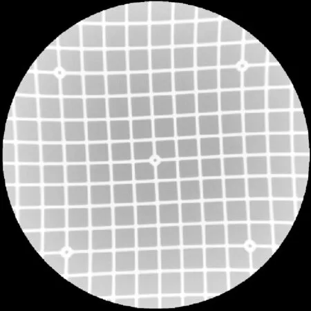
Fig.3 Distorted XRII image

During the implementation of experiments, the proposed algorithm was compared to the classical correction algorithms, such as the global polynomial correction model,local linear model L1 and nonlinear model L2. The classical global polynomial correction model[15]is shown as

The formulae of local linear model L1 and nonlinear model L2[15]are shown as

Model L1

(2)

Model L2

(3)

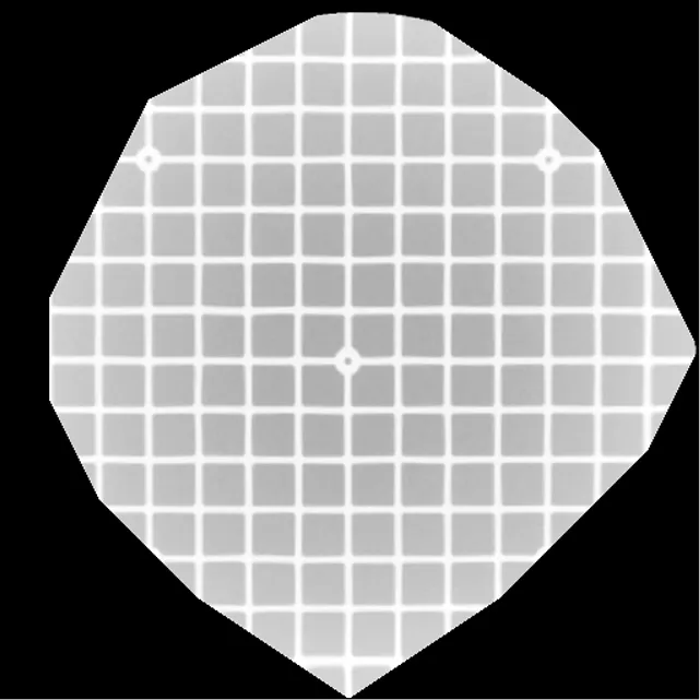
When models L1 and L2 are used to correct the distorted image, the distorted image is first divided into four sub-images along horizontal and vertical directions from its middle point. Then, every sub-image is corrected. The final image is obtained by fusing all the corrected sub-images. In the case of the same center, Fig.4 shows the corrected images using different correction algorithms. Correspondingly, Fig.5 illustrates the corrected images using all the correction algorithms when their centers do not coincide.

From Fig.3, the S-distortion and pillow distortion can be clearly found in the acquired XRII images. After the images were corrected using DTI, the S-distortion and pillow distortion no longer existed in the corrected images (see Fig.4(a) and Fig.5(a)). From Fig.4(a) and Fig.5(a), we can see that the corrected images are not very exact. The cause for the phenomenon is that the extracted control points mainly concentrate on the center position. Naturally, the phenomenon does not affect forming the relationship between the distorted image and the ideal image. Fig.4(b) and Fig.5(b) are the corrected images using the quartic polynomial. As can be seen from Fig.4(b) and Fig.5(b), the S-distortion does not exist and pillow distortion exists in part. As for Fig.4(c), Fig.4(d), Fig.5(c) and Fig.5(d), using local linear

(a)

(b)

(c)

(d)

(a)

(b)

(c)

(d)

model L1 and nonlinear model L2, there is S-distortion and pillow distortion to some extent. Moreover, the corrected image is broken into two images in Fig.4(c) with the corrected model L1. These phenomena further illustrate that the correction effect of the global correction algorithm is better than that of the local correction algorithm.

2.3 Quantitative comparison

In experiments, the correction accuracies of all correction algorithms are compared. Here, the correction algorithms include the global quartic polynomial correction algorithm, the local linear correction algorithm (model L1) and the nonlinear correction algorithm (model L2) and the DTI correction algorithm. Image distortion correction accuracy is judged using two indices, root mean square distances (RMSD) and standard deviation (STD). Their corresponding formulae are as follows:

(4)

(5)

wheredi=((x(i)-corrx(i))2+(y(i)-corry(i))2)1/2ordi=((xcenter(i)-corrx(i))2+(ycenter(i)-corry(i))2)1/2. RMSD is the root mean square error between computed control point’s coordination values in the ideal image and the corrected control point’s coordination values in the corrected image. The smaller RMSD implies a better correction effect. When RMSD equals zero, the interpolated surface passes though the control points in the ideal image. In this case, the correction effect is the best.

Tab.2 gives the correction accuracies of various correction algorithms when centers between the corrected image and the ideal image coincide. Correspondingly, when the centers between the distorted image and the ideal image do not coincide, the correction accuracies are listed in Tab.3. The RMSE and STDE of model L1 and model 2 are computed as follows. First, the RMSE and STDE of every sub-image are computed. Then, the RMSE and STDE summation of all the sub-images are computed. Finally, the final RMSE and STDE are calculated by averaging the summation.

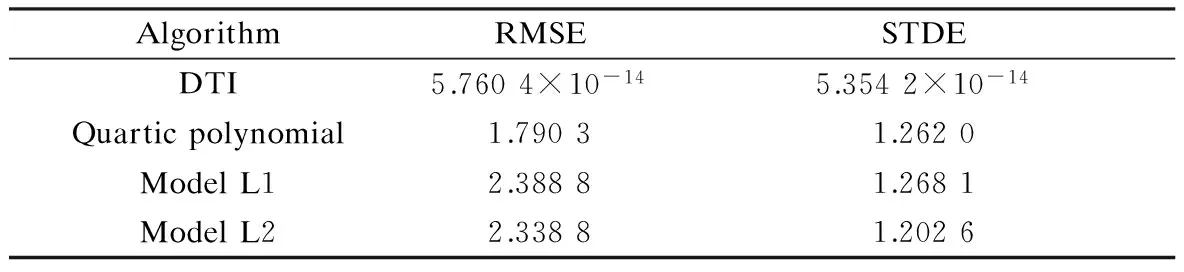
Tab.2 Correction accuracy with the same center

Tab.3 Correction accuracy with different centers

The RMSE and STDE between the corrected image using model L1 and the ideal image are 2.388 8 and 1.268 1 whether they have the same center or not. The two values become 2.338 8 and 1.202 6 whether they have the same center or not, after the model L2 is used to correct the distorted images. After global quartic polynomial correction, RMSE and STDE become 1.790 3 and 1.262 0 (The two images have the same center) and 1.770 3 and 1.269 9 (The two images have different centers), respectively. After using the correction algorithm proposed in this paper, RMSE and STDE become 5.760 4×10-14and 5.354 2×10-14(The two images have the same center) and 2.489×10-13and 2.449 8×10-13(The two images have different centers), respectively. These results prove that the proposed algorithm outperforms the classical global polynomial correction algorithm and the local linear correction algorithm (model L1) and the nonlinear correction algorithm (model L2).

3 Conclusion

The distorted XRII image can bring about adverse effects for subsequent courses. In this paper, a DTI algorithm based on the classical algorithms is proposed to correct the distorted images. Experimental results show that the proposed algorithm can not only effectively correct the distorted XRII images, but also bring about better results than the classical correction algorithms. To demonstrate its reliability and validity, in the future, we will apply the algorithm to clinical data and compare it with the classical algorithms.

[1]Lee K, Lee K M, Park M S, et al. Measurements of surgeons’ exposure to ionizing radiation dose during intraoperative use of C-arm fluoroscopy [J].Spine, 2012, 37(14): 1240-1244.

[2]Kothary N, Abdelmaksoud M H, Tognolini A, et al. Imaging guidance with C-arm CT: prospective evaluation of its impact on patient radiation exposure during transhepatic arterial chemoembolization[J].JournalofVascularandInterventionalRadiology, 2011, 22(11): 1535-1543.

[3]Yaniv Z. Evaluation of spherical fiducial localization in C-arm cone-beam CT using patient data [J].MedicalPhysics, 2010, 37(11): 5298-5305.

[4]Yan Shiju, Wang Chengtao, Ye Ming. A method based on moving least squares for XRII image distortion correction [J].MedicalPhysics, 2007, 34(11): 4194-4206.

[5]Holdsworth D W, Pollmann S I, Nikolov H N, et al. Correction of XRII geometric distortion using a liquid-filled grid and image subtraction[J].MedicalPhysics, 2005, 32(1): 55-64.

[6]Yan Shiju, Qian Liwei. XRII image distortion correction

for C-arm-based surgical navigation system [J].JournalofBiomedicalEngineering, 2010, 27(3): 548-551. (in Chinese)

[7]Li Yuanjin, Luo Limin, Zhang Pengcheng, et al. Distortion correction of XRII image based on calibration grid characteristic and Biharmonic interpolation[J].JournalofSoutheastUniversity:NaturalScienceEdition, 2011, 41(6): 1213-1218. (in Chinese)

[8]Cerveria P, Forlani C, Borghese N A, et al. Distortion correction for X-ray image intensifier: local unwarping polynomials and RBF neural networks [J].MedicalPhysics, 2002, 29(8): 1759-1771.

[9]Fink M, Haunert J H, Spoerhase J, et al. Selecting the aspect ratio of a scatter plot based on its Delaunay triangulation [J].IEEETransactionsonVisualizationandComputerGraphics, 2013, 19(12): 2326-2335.

[10]Gao Z, Yu Z, Holst M. Feature-preserving surface mesh smoothing via suboptimal Delaunay triangulation [J].GraphModels, 2013, 75(1): 23-38.

[11]Gao Z, Yu Z, Holst M. Quality tetrahedral mesh smoothing via boundary-optimized Delaunay triangulation [J].ComputerAidedGeometricDesign, 2012, 29(9): 707-721.

[12]Wang Jiayao.Thetheoryofspatialinformationsystem[M]. Beijing: Science Press, 2001: 172-186. (in Chinese)

[13]Wu Xiaobo, Wang Shixin, Xiao Cunsheng. A new study of Delaunay triangulation creation [J].ActaGeodaeticaEtAcrtographicaSinica, 1999, 28(1): 28-35.

[14]Li Yuanjin, Luo Limin, Zhang Quan, et al. The algorithm of calibration grid marker projection identification and coordinates data extraction [J].ComputerApplicationandSoftware, 2012, 29(5): 50-52, 63. (in Chinese)

[15]Gronenschild E. Correction for geometric image distortion in the X-ray imaging chain:local technique versus global technique [J].MedicalPhysics, 1999, 26(12): 2602-2616.

Delaunay三角网插值在XRII图像扭曲校正中的应用

李元金1, 2舒华忠1罗立民1陈 阳1王 涛2岳座刚2

(1东南大学影像与科学技术实验室, 南京 210096)(2滁州学院计算机与信息工程学院, 滁州 239000)

针对扭曲的影像加强器(X-ray image intensifier, XRII)图像对后继工作产生不利影响的问题,提出使用Delaunay三角网插值对扭曲的XRII图像进行校正.首先分析了XRII图像扭曲的原因、经典的校正方法和Delaunay三角网插值;然后,使用程序流程图对算法过程进行了解释.最后,通过实验来证明所提算法的有效性和可行性.实验结果表明:在中心对齐时,使用Delaunay三角插值方法校正后的XRII图像网格线交叉点坐标值与理想校正靶网格线交叉点坐标值的残留误差和标准误差分别为5.760 4×10-14和 5.354 2×10-14,使用经典的全局四次多项式、模型L1和模型L2校正之后残留误差和标准误差分别为 1.790 3, 2.388 8, 2.338 8和1.262 0, 1.268 1, 1.202 6;在中心不对齐时,使用Delaunay三角插值方法校正后的XRII图像网格线交叉点坐标值与理想校正靶网格线交叉点坐标值的残留误差和标准误差分别为2.489×10-13和 2.449 8×10-13,使用经典的全局四次多项式、模型L1和模型L2校正后残留误差和标准误差分别为1.770 3,2.388 8,2.338 8和1.269 9,1.268 1,1.202 6.

XRII图像; Delaunay三角插值; 扭曲校正; C臂X机

TP391.41

s：The Natural Science Foundation of Anhui Province (No.1308085MF96), the Project of Chuzhou University (No.2012qd06, 2011kj010B), the Scientific Research Foundation of Education Department of Anhui Province (No.KJ2014A186), the National Basic Research Program of China (973 Program) (No.2010CB732503).

：Li Yuanjin, Shu Huazhong, Luo Limin, et al. Application of the Delaunay triangulation interpolation in distortion XRII image[J].Journal of Southeast University (English Edition),2014,30(3):306-310.

10.3969/j.issn.1003-7985.2014.03.009

10.3969/j.issn.1003-7985.2014.03.009

Received 2014-02-09.

Biographies：Li Yuanjin(1976—), male, doctor, associate professor; Shu Huazhong (corresponding author), male, doctor, professor, shu.list@seu.edu.cn.