Xie Jiaye Zhou Houxing Mu Xing Hua Guang Li Weidong Hong Wei

(State Key Laboratory of Millimeter Waves, Southeast University, Nanjing 210096, China)



P-FFT and FG-FFT with real coefficients algorithm for the EFIE

Xie Jiaye Zhou Houxing Mu Xing Hua Guang Li Weidong Hong Wei

(State Key Laboratory of Millimeter Waves, Southeast University, Nanjing 210096, China)

In order to reduce the storage amount for the sparse coefficient matrix in pre-corrected fast Fourier transform (P-FFT) or fitting the Green function fast Fourier transform (FG-FFT), the real coefficients are solved by improving the solution method of the coefficient equations. The novel method in both P-FFT and FG-FFT for the electric field integral equation (EFIE) is employed. With the proposed method, the storage amount for the sparse coefficient matrix can be reduced to the same level as that in the adaptive integral method (AIM) or the integral equation fast Fourier transform (IE-FFT). Meanwhile, the new algorithms do not increase the number of the FFTs used in a matrix-vector product, and maintain almost the same level of accuracy as the original versions. Besides, in respect of the time cost in each iteration, the new algorithms have also the same level as AIM (or IE-FFT). The numerical examples demonstrate the advantages of the proposed method.

real coefficients; complex coefficients; pre-corrected fast Fourier transform (P-FFT); fitting the Green function fast Fourier transform (FG-FFT)

The integral equation (IE) formulation in conjunction with the method of moments (MoM) is a popular tool for the analysis of electromagnetic scattering from and/or radiation by an object. However, even using an iterative method,O(N2) operations per iteration is also needed, whereNis the number of unknowns. Thus, the application of the tool to electrically large complex structures is restricted.

Many fast algorithms have been proposed to speed up the evaluation of matrix-vector products and to simultaneously reduce the memory requirement. Here, we focus on the FFT-based methods in which the FFT is employed to speed up the matrix-vector products.

The CG-FFT is the pioneer of the FFT-based method. After that, several advanced methods were developed. The idea of the AIM[1]is to project the local basis functions onto the node basis functions which are defined as the nodes of a uniform Cartesian grid. The projection coefficients are obtained by matching the high order multi-pole moments. The principle of the P-FFT[2]is similar to that of the AIM, but the projection coefficients are obtained by matching the potentials rather than the high order multipole moments. P-FFT possesses higher accuracy compared with the AIM and hence can be applied to a relatively coarse grid[3-4]. Unlike the AIM and P-FFT, both the IE-FFT[5]and the FG-FFT[3]are used to represent the Green function with the values at the nodes of a uniform Cartesian grid. IE-FFT uses the Lagrange Interpolation, while FG-FFT employs the fitting technique. So far, the FFT-based methods have many applications[6-9].

Generally, the AIM and IE-FFT have the same accuracy level[4], so do the P-FFT and FG-FFT[3]. However, the sparse coefficient matrices in the latter two methods are complex matrices for non-zero frequency cases, while those in the former two methods are always real matrices. In other words, the storage amount for the sparse coefficient matrix in P-FFT (or in the FG-FFT) is twice as large as that in the AIM (or in IE-FFT) for non-zero frequency cases. Therefore, reducing memory requirements for the sparse coefficient matrices of the P-FFT and FG-FFT is a significant project.

In this paper, a method with real coefficients in both the P-FFT and the FG-FFT for the EFIE is proposed. With the proposed method, the storage amount for the sparse coefficient matrix in the P-FFT (or in FG-FFT) can be reduced to the same amount as in the AIM (or in IE-FFT) for non-zero frequency cases. The new algorithms do not increase the number of the FFTs used in a matrix-vector product, and maintain almost the same level of accuracy as the original versions. In addition, in respect of the time cost in each iteration, the new algorithms have also the same amount as the AIM (or IE-FFT). In this paper,λalways denotes the wavelength in the free space.

1 Formulation

1.1 Projection coefficients

In the CP-FFT, the projection coefficientsΛn,u’s andκn,u’s are obtained by means of the following overdetermined equations[2]:

(1)

(2)

Eqs.(1) and (2) can be rewritten as

AX(p)=Φ(p)p=1,2,3,4

(3)

Whenp=1,2,3,

Whenp=4,

and whenp=4,X(p)={κn,u}.

1.2 Coefficients representation

(4)

Eq.(4) can be rewritten as

AX(5)=Φ(5)

(5)

1.3 Real coefficients finding

Eqs.(3) and (5) have the unified form as

AY=Ψ

(6)

Now, letA=Are+jAimandΨ=Ψre+jΨim. WhenY∈R|Cn|×1is imposed on Eq.(6), Eq.(6) is equivalent to the following form:

(7)

Therefore, using Eq.(7) instead of Eq.(6) in P-FFT and FG-FFT can produce real coefficients, leading to the RP-FFT and the RFG-FFT. Here, the frames of P-FFT and FG-FFT are unchanged, and hence the number of the FFTs used in a matrix-vector product is unchanged also.

2 Numerical Results

2.1 Accuracy examination

To compare the accuracy of the new real coefficients algorithms with that of the original versions, we provide an example and examine the relative errors of the impedance matrices. The relative error (RE) is defined as

(8)

Example 1 A PEC sphere with radiusλ

For a PEC sphere of radiusλ, the REs of the impedance matrices from the CP-FFT, the CFG-FFT, the RP-FFT and the RFG-FFT are examined. In this example, the number of unknowns is 4 773. The grid spacings are selected ashx=hy=hz=0.2λ, and the expansion order is selected asM=2. The REs of the impedance matrices from these methods are recorded in Tab.1. It is seen that the new algorithms maintain almost the same level of accuracy as the original versions.

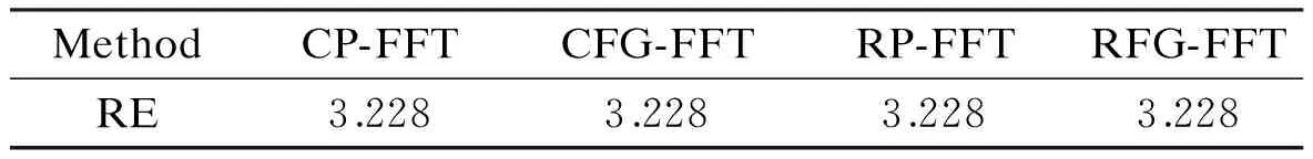
Tab.1 Relative errors of impedance matrices 10-3

2.2 Efficiency examination

Here, all the calculations are performed with double precision. The 8-kernel CPU parallel computation is used and the FFT codes are from the FFTW[10]. In P-FFT and FG-FFT, the grid spacings are selected to be equal, i.e.,hx=hy=hz=h, and the expansion order is selected asM=2. When the scattering from a perfect electric conductor (PEC) object is to be calculated, the surface of the object is always discretized with about 10 elements per wavelength, and the RWG basis functions are applied. Besides, the root mean square error (RMSE) of the RCS is defined as

(9)

whereLis the number of the azimuth angle samples, and RCSkcorresponds to thek-th azimuth angle sample.

2.2.1 A PEC sphere with radius 5.0λ

The scattering from a PEC sphere of radius 5.0λis calculated by IE-FFT, the RFG-FFT and the CFG-FFT, and compared with the Mie series solution (as the bench mark). In this example, the number of unknowns is 113 421. The bi-static RCS curves obtained are shown in Fig.1. It is seen from Fig.1 that the numerical solutions from both the RFG-FFT and the CFG-FFT agree well with the Mie series solution, but that from IE-FFT is obviously different from the Mie series solution in the vicinity of the backward scattering angle. The RMSE, the time cost and the storage amount are recorded in Tab.2, Example A.

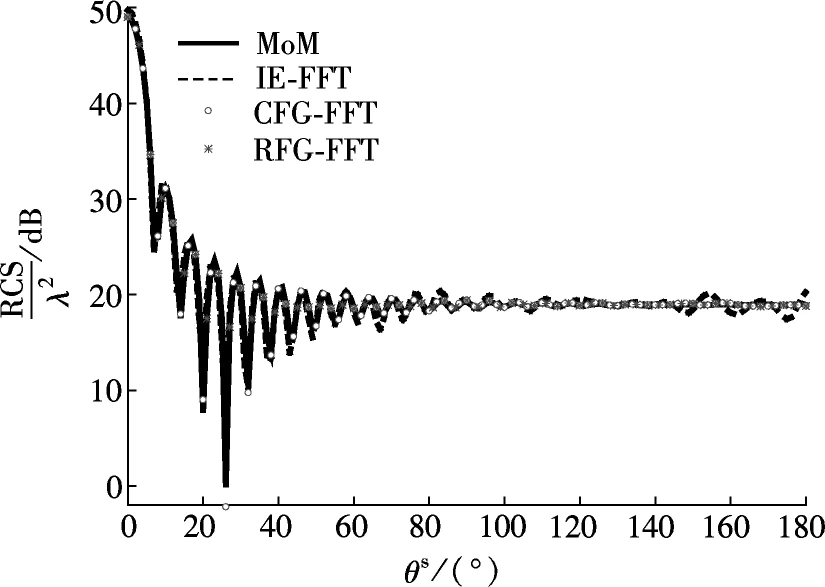
Fig.1 RCS curves of the PEC sphere with h=0.2λ and M=2(φin=0°, θin=0°, φs=0°)

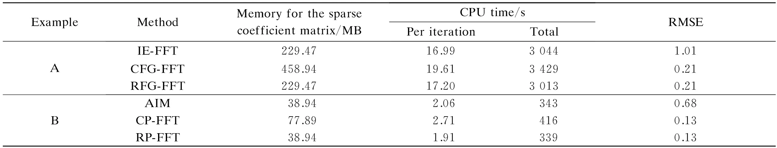
ExampleMethodMemoryforthesparsecoefficientmatrix/MBCPUtime/sPeriterationTotalRMSEAIE-FFT229.4716.9930441.01CFG-FFT458.9419.6134290.21RFG-FFT229.4717.2030130.21BAIM38.942.063430.68CP-FFT77.892.714160.13RP-FFT38.941.913390.13

2.2.2 A PEC folded plate

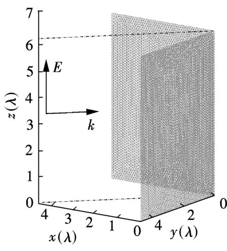
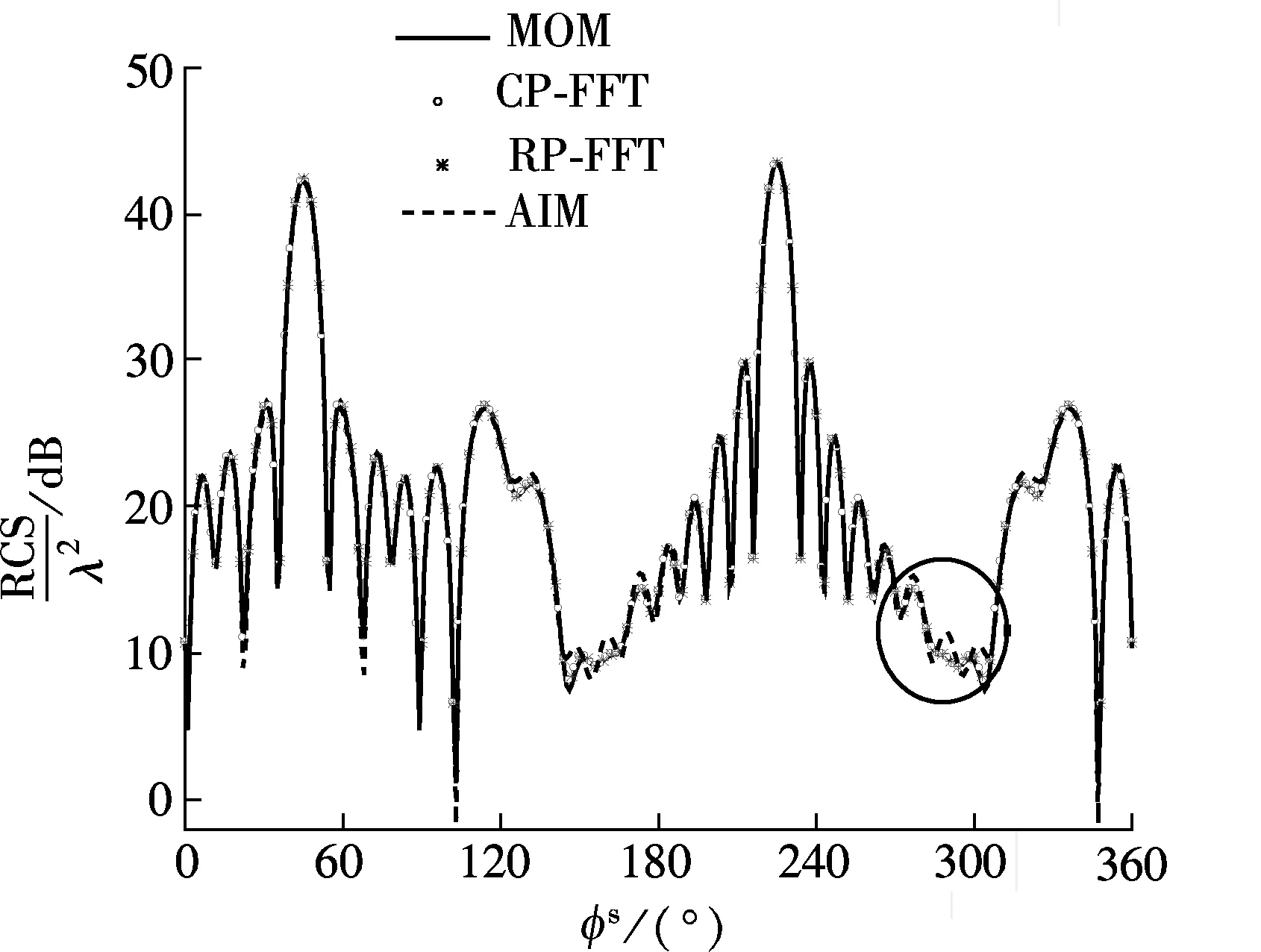
A PEC folded plate with an dihedral angle of 90°is shown in Fig.2(a), and each sub-plate has the dimensions 4.687 5λ×6.25λ. The direction and polarization of the incident plane wave are also shown in Fig.2(a). The scattering from this object is calculated by AIM, the CP-FFT and the RP-FFT, and compared with the MoM solution (as the benchmark). In this example, the number of unknowns is 19 565. The bi-static RCS curves obtained are shown in Fig.2(b) and a drawing of partial enlargement is shown in Fig.2(c). It can be seen from Figs.2(b) and (c) that the numerical solutions from both the CP-FFT and the RP-FFT and the MoM solution coincide very well, but that from AIM is obviously different from the MoM solution at some azimuth angle samples.

(a)

(b)

(c)

Fig.2 RCS curves of the PEC folded plate withh=0.2λandM=2 (φin=225°,θin=90°,φs=90°). (a) A PEC folded plate; (b) RCS curves of the PEC folded plate; (c) A drawing of partial enlargement

The RMSE, the time cost and the storage amount are recorded in Tab.2, Example B. It can be concluded from the above two examples that in respect of both the storage amount for the sparse coefficient matrix and the time cost in each iteration, the RP-FFT and the RFG-FFT have the same level as AIM (or IE-FFT).

3 Conclusion

In this paper, the modified P-FFT and FG-FFT (called RP-FFT and RFG-FFT, respectively) that have real coefficients for the EFIE are established. Compared with the original versions, the new algorithms maintain the same number of the FFTs used in a matrix-vector product and possess almost the same level of accuracy. Besides, each of the two new algorithms needs only the same storage amount for the sparse coefficient matrix as AIM (or IE-FFT); that is, the storage amount for the sparse coefficient matrix is reduced to half the original amount of storage.

[1]Bleszynski M, Bleszynski E, Jaroszewicz T. AIM: adaptive integral method for solving large-scale electromagnetic scattering and radiation problems [J].RadioSci, 1996, 31(3): 1225-1251.

[2]Nie X C, Li L W, Yuan N. Precorrected-FFT algorithm for solving combined field integral equations in electromagnetic scattering [J].JElectromagnWavesAppl, 2002, 16(8): 1171-1187.

[3]Xie J Y, Zhou H X, Hong W, et al. A novel FG-FFT method for the EFIE [C]//2012InternationalConferenceonComputationalProblem-Solving. Leshan, China, 2012:111-115.

[4]Yang K, Yilmaz A E. Comparison of pre-corrected FFT/adaptive integral method matching schemes [J].MicrowOptTechLett, 2011, 53(6): 1368-1372.

[5]Yin J, Hu J, Nie Z P, et al. Floating interpolation stencil topology-based IE-FFT algorithm [J].ProgElectromagnResearchM, 2011, 16: 245-259.

[6]Wu M F, Kaur G, Yilmaz A E. A multiple-grid adaptive integral method for multi-region problems [J].IEEETransAntennasPropag, 2010, 58(3): 1601-1613.

[7]Xie J Y, Zhou H X, Kong W B, et al. A 2-level AIM for solving EM scattering from electrically large objects [C]//2010InternationalConferenceonComputationalProblem-Solving. Lijiang, China, 2010: 9-11.

[8]An X, Lu Z Q. Application of IE-FFT with combined field integral equation to electrically large scattering problems [J].MicrowOptTechLett, 2008, 50(7): 2561-2566.

[9]Xie J Y, Zhou H X, Li W D, et al. IE-FFT for the combined field integral equation applied to electrically large objects [J].MicrowOptTechLett, 2012, 54(2): 891-896.

[10]Frigo M, Johnson S. FFTW manual [EB/OL].(2011-07-26)[2013-09-06]. http://www.fftw.org/.

针对电场积分方程的P-FFT和FG-FFT实系数算法

谢家烨 周后型 牟 星 华 光 李卫东 洪 伟

(东南大学毫米波国家重点实验室, 南京 210096)

为了减少预修正快速傅立叶变换算法(P-FFT)或拟合格林函数快速傅立叶变换算法(FG-FFT)的稀疏系数矩阵所需的存储空间,通过改进系数方程的求解方法,获得实系数解.并将改进的求解方法与P-FFT和FG-FF相结合用于计算电场积分方程.所提方案将P-FFT/FG-FFT的稀疏系数矩阵的存储量降到自适应积分方法(AIM)/积分方程快速傅立叶变换算法(IE-FFT)相同水平的同时,未增加矩阵向量积所需FFT的次数,并保持原有算法的精度水平.此外,在每次迭代的时间耗费方面,新方案与AIM/IE-FFT相当.数值实验证实了新方案的上述优点.

实系数;复系数;预修正快速傅立叶变换算法;拟合格林函数快速傅立叶变换算法

TN011

The National Basic Research Program of China (973 Program) (No.2013CB329002).

：Xie Jiaye, Zhou Houxing, Mu Xing, et al. P-FFT and FG-FFT with real coefficients algorithm for the EFIE[J].Journal of Southeast University (English Edition),2014,30(3):267-270.

10.3969/j.issn.1003-7985.2014.03.002

10.3969/j.issn.1003-7985.2014.03.002

Received 2014-02-25.

Biographies：Xie Jiaye (1980—), male, doctor, lecturer; Zhou Hou-xing (corresponding author), male, doctor, professor, hxzhou@emfield.org.