ZHANG Hong-sheng (张洪生), JIA Hai-qing (贾海青)

College of Ocean Science and Engineering, Shanghai Maritime University, Shanghai 201306, China,

E-mail: hszhang@shmtu.edu.cn

GU Jun-bo (辜俊波)

East China Electric Power Design Institute，China Power Engineering Consulting Group, Shanghai 200063, China

LI Peng-hui (李朋辉)

College of Ocean Science and Engineering, Shanghai Maritime University, Shanghai 201306, China

Numerical simulation of the internal wave propagation in continuously densitystratified ocean*

ZHANG Hong-sheng (张洪生), JIA Hai-qing (贾海青)

College of Ocean Science and Engineering, Shanghai Maritime University, Shanghai 201306, China,

E-mail: hszhang@shmtu.edu.cn

GU Jun-bo (辜俊波)

East China Electric Power Design Institute，China Power Engineering Consulting Group, Shanghai 200063, China

LI Peng-hui (李朋辉)

College of Ocean Science and Engineering, Shanghai Maritime University, Shanghai 201306, China

(Received February 20, 2014, Revised June 23, 2014)

A numerical model is proposed to simulate the internal wave propagation in a continuously density-stratified ocean, and in the model, the momentum equations are derived from the Euler equations on the basis of the Boussinesq approximation. The governing equations, including the continuity equation and the momentum equations, are discretized with the finite volume method. The advection terms are treated with the total variation diminishing (TVD) scheme, and the SIMPLE algorithm is employed to solve the discretized governing equations. After the modeling test, the suitable TVD scheme is selected. The SIMPLE algorithm is modified to simplify the calculation process, and it is easily made to adapt to the TVD scheme. The Sommerfeld’s radiation condition combined with a sponge layer is adopted at the outflow boundary. In the water flume with a constant water depth, the numerical results are compared to the analytical solutions with a good agreement. The numerical simulations are carried out for a wave flume with a submerged dike, and the model results are analyzed in detail. The results show that the present numerical model can effectively simulate the propagation of the internal wave.

internal wave, continuously density-stratified fluid, finite volume method, SIMPLE algorithm, numerical simulation

Introduction

Internal waves can be found within subsurface layers of the sea density-stratified due to temperature and salinity variations. The largest vertical displacement of the internal waves is within the fluid, as is opposed to that of the surface waves. Internal waves and their side effects were widely studied[1-3]and it is shown that they can significantly influence the oceanic current undersea circulation, the antisubmarine warfare operations, the safety of ocean structures, and even the feeding habits of marine animals.

There were a large number of numerical simulations for the internal waves, including their generation, propagation, and dissipation[4-8]. A two-layer model[9]and a multi-layer model[4]were proposed, three-dimensional primitive equations were applied in numerical ocean models[10,11], such as the Center for Water Research Estuary and Lake Computer Modelology (CWR-ELCOM)[12]and princeton ocean model (POM , Blumbery and Mellor,1987), which were developed on the basis of the hydrostatic assumption that is suitable for the case where the horizontal length scale is large compared with the vertical length scale. A numerical model will be developed in this paper, to consider both the hydrostatic and hydrodynamic processes where the horizontal and vertical scales are of a similar order.

The SIMPLE algorithm[13]was developed by Patankar and Spalding in 1972, and was employed to numerically simulate various fluid flows[14-16]. The focus of this paper is to develop a numerical model that can numerically simulate the propagation of the internal waves in a continuously density-stratified ocean with a variable bottom topography. The SIMPLE algorithm will be employed to solve the governing equations, including the continuity equation and the momentum equations, which are derived from the Euler equations for the two-dimensional incompressible fluid on the basis of the Boussinesq approximation. The governing equations are discretized with the finite volume method. To achieve a second order accuracy, the TVD(Total Variation Diminishing) scheme[17]is used to treat the advection terms. The SIMPLE algorithm is modified to make it easily adapt to the TVD scheme and to improve the calculation speed. In the numerical model, the sponge layer combined with the Sommerfeld (1949)’s radiation condition is used at the outflow boundary and the model is verified in the water flume with a constant water depth and with a variable bottom topography. In the end, some conclusions are presented.

1. Governing equations

The fluid is assumed to be inviscid and incompressible, and the Coriolis force is neglected. A Cartesian coordinate system (x ,y) is adopted, with the -z axis pointing upward from the still water level. The equations for the two-dimensional flow are expressed as:

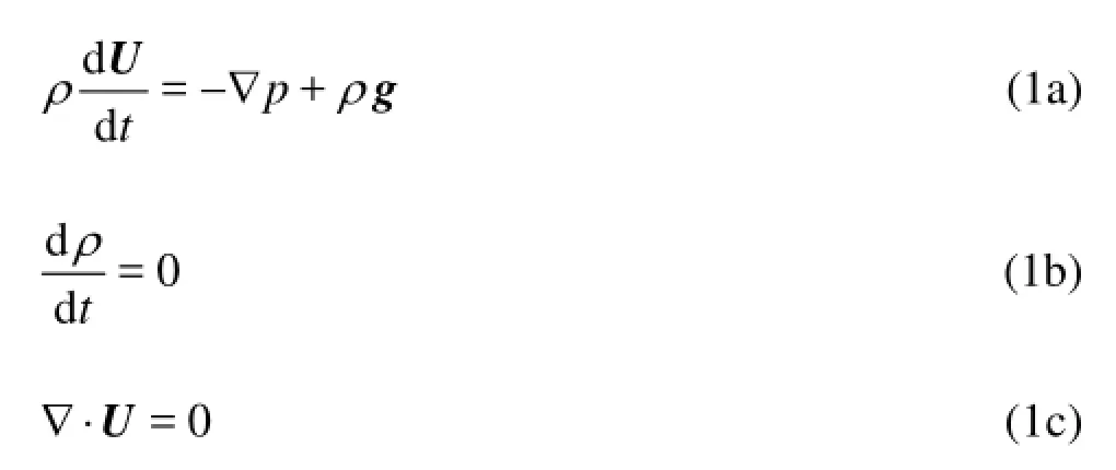
where the velocity vector U=(u, w), t is the time, g is the gravitational acceleration, ρ is the density of the sea water, p is the pressure, and ∇=(∂/∂x,∂/∂z).

The density ρ is split into two parts

where ρ0(z) is the constant reference density, and ρ＇(x, z, t ) is the perturbation density. Substitution of Eq.(2) into Eq.(1a) leads to

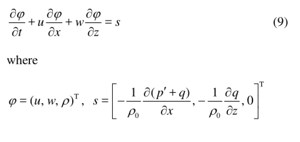
Equations (8a)-(8d) are the governing equations. Equations (8a)-(8c) can be expressed in the form of a two-dimensional convection-diffusion equation with a source term

2. Numerical model

2.1The Arakawa C-grid

Figure 1 shows the Arakawa C-grid adopted in this paper. In z- and x-directions, the node indices are termed i and j, respectively, where i=1,2,…, nz and j=1,2,…,nx.This indicates that the nodal coordinates are z=(i-1)Δz and x=(j-1)Δx, where Δz and Δx are the grid sizes in z- and x-directions, respectively. The velocity in x-direction, u, is defined on the point (i+1/2,j+1/2), the velocity in z-direction, w, is defined on the grid point (i, j), the scalar functions, such as ρ and q are defined on the point (i+1/2,j). Moreover, in order to deal with the varied sea bottom, a logical variable wet is defined on the point (i+1/2,j). It indicates that the control volume, including the point (i+1/2,j), belongs to solid or liquid.

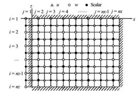
Fig.1 Sketch of Arakawa C-grid

2.2Discretization of governing equations

Integrating Eq.(9) in time and over a two-dimensional control volume(in -x z plane ) as shown in Fig.2, we obtain

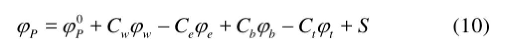
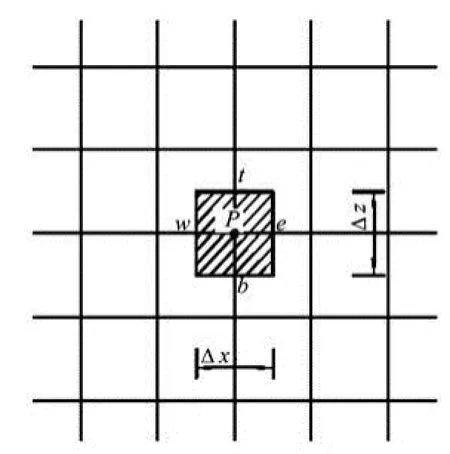
Fig.2 Sketch of the computational grid for finite volume method

When the advection term is discretized, the second-order spatial accuracy can be achieved by the use of the total variation diminishing (TVD) scheme. First of all, the velocity variables u and w are split into two parts:

The Courant numbers and φ over each face should also be split, Eq.(10) is then expressed as

For the TVD scheme employed in this paper, the flux-face values are computed with the upwind values plus a higher-order term with:

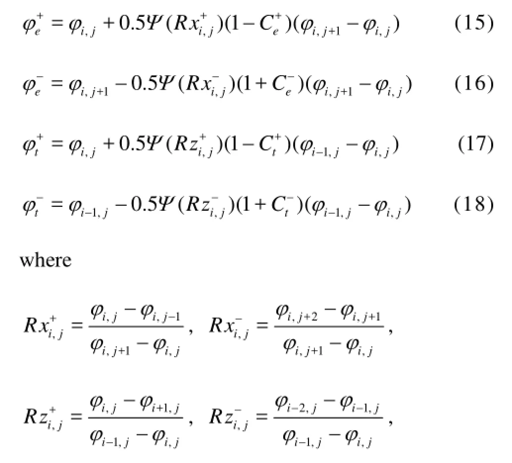
Ψ(R)=0 is a limiter function. Different limiters can lead to different TVD schemes.

Finally, the source term is discretized. For different variables, Eq.(10) are, respectively, expressed as:

In Eq.(19), the value of p＇ at the previous time is used because it varies slowly.

Equation (8d) is discretized by the backward-differencing in space

2.3Improvement of SIMPLE algorithm

The SIMPLE algorithm[13]is employed in this paper. The predicted velocity field is implicitly calculated in the original SIMPLE algorithm. However, it should be improved for two reasons. The first reason is that the pressure (,,)p x y t is split into three parts, therefore, the hydrostatic pressure corrections due to the density disturbance are involved in the present study, whereas, they are not involved in the original SIMPLE algorithm. The second reason is that the TVD scheme is employed. If the original SIMPLE algorithm is used directly, the calculation of the coefficients of Eqs.(19) and (20) would be complicated, and the limiter function Ψ(R)=0 could not be adapted easily.

In this paper, in order to explicitly calculate the predicted velocity field (u**,w**) at t=(n+1)Δt, the assumed velocity field (u*,w*) and the hydrodynamic pressure q*are given at the beginning of the iteration, and they are set as the corresponding values at t= nΔ t, respectively. Whereas, in the original SIMPLE algorithm, the predicted velocity field (u**,w**) is implicitly calculated, thus the two equations should be solved. The present approach can simplify the calculation process and be adapted to the use of the limiter function easily. Therefore, the present approach will increase the number of iterations. However, the modeling test shows that the calculation speed is increased as a whole, rather than otherwise. Thus, based on Eqs.(19) and (20), the velocity field (u**,w**) is expressed as:

The predicted velocity field (,)uw****cannot often satisfy the continuity equation unless the predicted non-hydrostatic pressure field is correct. Assume a new non-hydrostatic pressure field q**, which is used to replace q*in Eqs.(23) and (24), the corrected velocity field can be obtained:

The corrected velocity field (u***,w***) is further assumed to satisfy the continuity equation. Subtraction of Eqs.(23) and (24) from Eqs.(25) and (26), respectively, leads to:

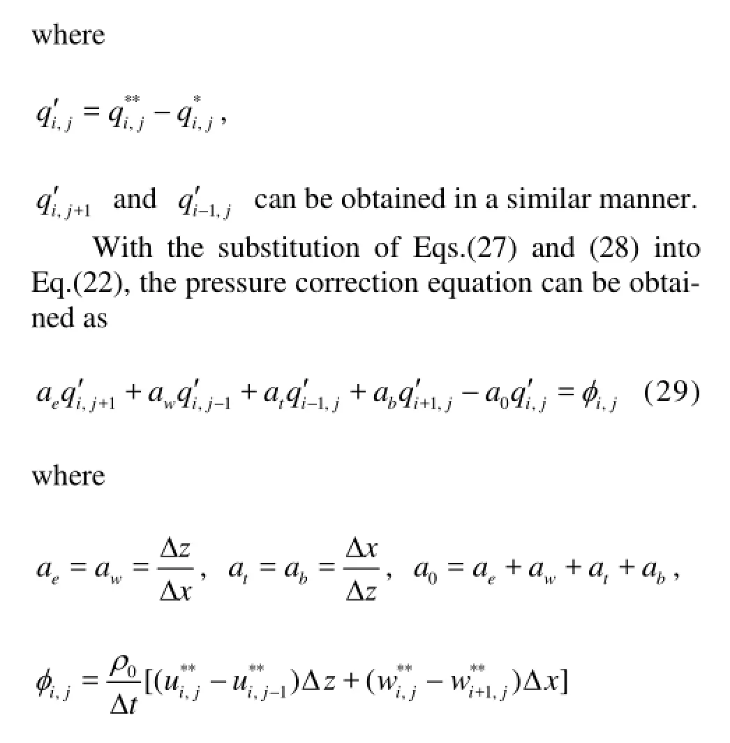
Solving Eq.(29), qi＇,jis obtained. It is substituted into Eqs.(27)-(28), the corrected velocity field (u***,w***) and the corrected non-hydrostatic pressure q**are then obtained. If

where ε is the convergence criterion (chosen as 1.0× 10-5m/s in this paper), the velocity field at the present time t=(n+1)Δt, (u, w), should be equal to (u***, w***). Otherwise, we let (u*,w*)=(u***,w***) and q*=q**, and the calculation process is then repeated until the convergence criterion is satisfied.

In the end, the velocity field at the present time t=(n+1)Δt, (u, w), and the density field at the previous time t=nΔ t, ρ0, are used to calculate adv(ρ) in Eq.(21) . The density field at t=(n+1)Δt, ρ, can be obtained. p＇ can be calculated by

where h is the water depth. This step is specially devised for the problem of internal waves considered in this paper, and is not included in the original SIMPLE algorithm.

2.4Boundary conditions

The uniform incoming velocity field is directly specified according to the linear internal wave theory[1]. The sea floor is assumed to be a solid boundary, and the sea surface is assumed to be a rigid lid. The Sommerfeld (1949)’s radiation condition combined with a sponge layer is adopted on the outflow boundary. The governing equations in the sponge layer are

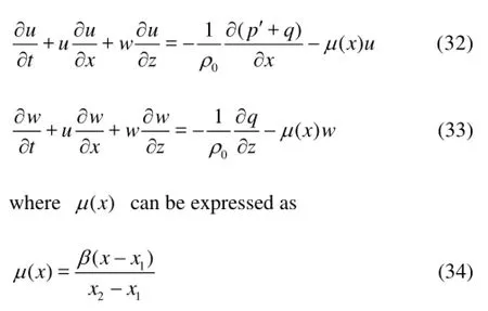
After initial model tests, β is chosen as 0.05, the head of the sponge layer is on the section x=x1, and the back end is on the section x=x2, the length of the sponge layer is x2-x1, and it can be chosen in the range from 1 to 2 wavelengths.

As mentioned above, a logical variable wet is defined on the grid (i+1/2,j). If weti+1/2,j=true, the control volume including the grid (i+1/2,j) is full of fluid, otherwise, it is solid. A row of grid points should be added outside the sea floor and the sea surface, respectively, and the control volumes including the grid points (1/2,j) and (nz+1/2,j) are assumed to be solid. If a control volume is solid, the fluxes on its faces and the velocity components normal to its surfaces are equal to zero. The present approach can deal not only with the regular variable topography but also with the irregular variable topography. Of course, this leads to a step-like representation of the sea floor.

3. Model tests

3.1Propagation of internal wave in the water flume with constant depth

If the water is of uniform depth, ρ0(z) can be assumed as[1,2]

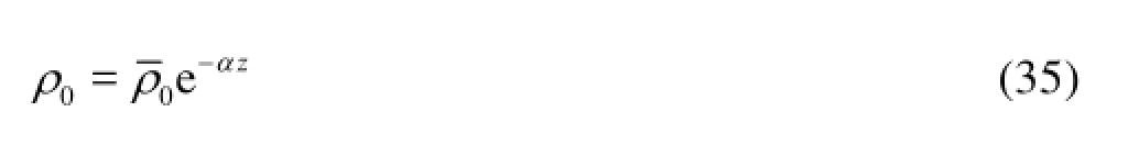
Fig.3 Calculated time series of density for Case 1 with different schemes at selected points

Fig.4 Calculated time series of density for Case 2 with different schemes at selected points

where ψ is the stream function, A is a coefficient relative to the amplitude of the internal wave, ω is the angular frequency, and k is the wave number.

From Eq.(36), the velocity fields can be expressed as:

Substitution of Eq.(2) into Eq.(8c) can approximately yield

Fig.5 Distributions of velocity vectors at t=8000s

Fig.6 Vertical profiles of velocities for x=500 m-700 m at t=8000s

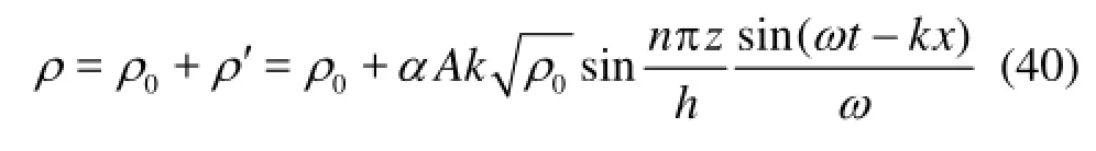
Equations (35) and (38) are substituted into Eq.(39), respectively, and the analytical solutions of density can then be expressed as

If Ψ(R)=0, the scheme reduces to the upwind scheme, which is accurate to the first-order in space and time. All other schemes are accurate to the second-order in both space and time. The calculated results for Cases 1 and 2 with the Superbee scheme and the upwind scheme are shown in Figs.3 and 4, respectively. From those figures, it is shown that the calculated amplitude of the density with the upwind scheme becomes smaller and smaller as the calculation time goes on. This is because the accuracy of the upwind scheme is not high enough. It is also found that the phase calculated with the upwind scheme is not in agreement with the theoretical one. Both the calculated amplitude of the density and the calculated phase with the Superbee scheme, however, are in good agreement with the theoretical ones. As mentioned above, it is obviously indicated that the accuracy of the calculatedresults with the Superbee scheme is better than that with the upwind scheme. Other schemes are used to obtain the density, velocity, and pressure fields, and similar results are obtained as those with the Superbee scheme. Therefore, the Superbee scheme is chosen as the limiter function in the present study.

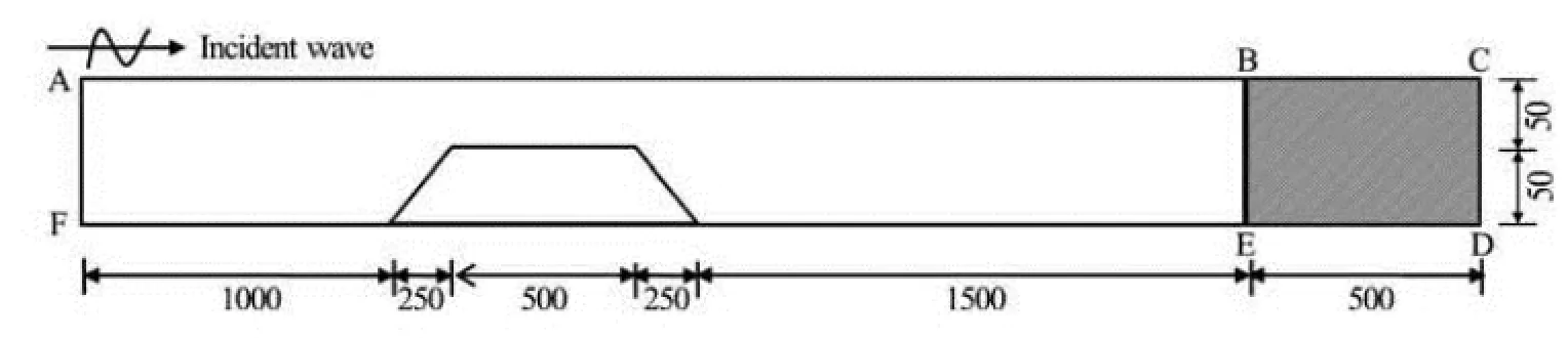
Fig.7 Sketch of the water flume with a submerged dike (m)

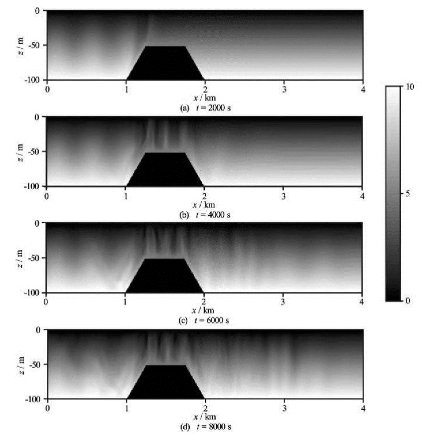
Fig.8 Distribution of the densities at different instants relative to those on the sea surface

The contours of the velocity vector at t=8000s are shown in Fig.5, where the velocity vectors form many rings. The contours of the velocity vector at different moments are compared, and it is found that the rings go forward with time. This indicates that the internal wave propagates forward. From Fig.5, it is also found that the vertical velocities at the sea surface and at the sea floor are equal to zero and they reach the maximum at the center of perpendicular lines. This is because the solid boundary conditions are applied at the upper and lower boundaries. The variation tendencies of the horizontal velocity are opposite to those of the vertical velocity. In fact, the above inferences can also be drawn from the theoretical solutions.

The calculated velocity distributions along the vertical sections from x=500 m to x=700 m are shown in Fig.6. From Fig.6 it may be concluded that the vertical velocities are the largest at the center of the vertical profiles, whereas they gradually decrease towards both the sea bottom and the free surface; the horizontal velocities are equal to zero at the center of the vertical profiles, whereas they gradually increasetowards both the sea bottom and the free surface. From the sea floor to the sea surface, the distributions of the vertical velocities follow a cosine function, whereas the distributions of the horizontal velocities follow a sinusoidal function. However, the amplitudes at different locations are different, and they also follow a sinusoidal (cosine) function.

3.2Propagation of internal wave over a submerged bar

The layout of the water flume with a submerged bar is shown in Fig.7. In the figure, the shadow region represents the sponge layer of 500 m in length, the still water depth is 100 m in the deep region and is reduced to 50 m on the top of the bar consisting of an upward slope of 1:5 and a 500 m horizontal crest followed by a down slope of 1:5. All the relevant model parameters are the same as those for Case 2 in the above subsection. The distributions of the relative densities with the benchmark value of the density at the sea surface are shown in Fig.8 at different moments. It is shown that the wavelength at the top of the bar is decreased, whereas the wavelength is increased in the lee of the bar. It is also indicated that the internal wave brings the water with high density to the top of the bar at the moment of t=4 000 s, 6 000 s and 8 000 s, and that the internal wave then acts as a “submarine blender”.

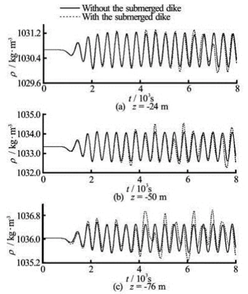
Fig.9 Time series of density at the points x=1000 m

The time series of the density at the toe of the front face and of the back face of the bar are shown in Figs.9 and 10 in the presence and the absence of the bar, respectively. In those figures, the solid line and the dashed line represent the numerical solutions in the presence and the absence of the bar, respectively. From Fig.9, it is found that the amplitudes of the density almost remain constant in the absence of the bar, and that the amplitudes of the density vary significantly in the presence of the bar. At a certain point, the time series of the density in the presence of the bar correspond to those in the absence of the bar during some period, and they then diverge from each other. Moreover, the shallower the water depth of some point, the longer the time during which the time series of the density in the presence of the bar correspond to those in the absence of the bar, and vice versa. This is because there will be more wave reflections and the reflections will occur earlier at the point of a greater water depth. From Fig.10, the moment at which the fluctuations at three points begin to be generated in the presence of the bar is later than that in the absence of the bar, and the amplitudes in the former case are smaller than those in the latter case. This is due to the shadowing effect of the bar. On the whole, the present numerical model can effectively simulate the propagation of the internal wave on a variable bottom topography.

Fig.10 Time series of density at the points x=2000 m

4. Conclusions

In the paper, a numerical model is developed for the propagation of the internal wave in the continuously density-stratified ocean. In the numerical model, the momentum equations among the governing equations are derived from the Euler equations for the twodimensional incompressible fluid on the basis of Boussinesq approximation. The governing equations, namely, the continuity equation and the momentum equations, are discretized with the finite volume method and solved with the SIMPLE algorithm, the TVDscheme is employed to evaluate the advection terms. In the original SIMPLE algorithm, the predicted velocity field is implicitly calculated, whereas it is explicitly calculated by assuming a velocity field in this paper. In doing so the calculation process can be simplified and the TVD scheme can easily be adapted. It is shown that although the present algorithm might increase the number of iteration steps, it is verified, according to the modeling tests, that the calculation speed of the present algorithm is faster than that of the original algorithm. Moreover, in the original SIMPLE algorithm, the hydrostatic pressure corrections due to the density disturbance are not included, whereas they are included and formulated in the present paper, as in the modified SIMPLE algorithm. The sponge layer combined with the Sommerfeld’s radiation condition is employed on the outflow boundary.

The present numerical model is verified in the water flume with a constant depth and a submerged dike. In the former case, the calculation results are in agreement with the analytical ones. In the latter case, the calculation results are analyzed in detail, and it is found that the calculation results can adequately reflect the effect of the submerged dike. Thus, the present numerical model can effectively simulate the propagation and transformation of the internal wave in the density-stratified ocean. The theoretical formula for the density is also derived for the two-dimensional flow in a continuously density-stratified ocean with a constant depth. It should be pointed out that in this paper, the bottom topography is implicitly defined by letting the velocity component normal to the solid boundaries be equal to zero. This leads to a step-like representation of the sea floor. Therefore, it is necessary that the governing equations are written in terrain-following coordinates in the vertical direction in the future work.

[1] PHILLIPS O. M. Dynamics of the upper ocean[M]. 2nd Edition, Cambridge, UK: Cambridge University Press, 1977.

[2] LIU Ying-zhong, MIAO Guo-ping. Advanced fluid mechanics[M]. 2nd Edition, Shanghai, China: Shanghai Jiao Tong University Press, 2002(in Chinese).

[3] GASTEL P. V., IVEY G. N. and MEULENERS M. J. et al. The variability of the large-amplitude internal wave field on the Australian North West Shelf[J]. Continental Shelf Research, 2009, 29(11): 1373-1383.

[4] FANG Guo-hong, LI Hong-yan and DU Tao. A layered 3-D numerical ocean model for simulation of internal tides[J]. Studia Marina Sinica, 1997, 38(1): 1-15(in Chinese).

[5] CAI S. Q., XIE J. S. and XU J. X. et al. Monthly variation of some parameters about internal solitary waves in the South China sea[J]. Deep-sea Research, 2014, 84: 73-85.

[6] LIU Guo-tao, SHANG Xiao-dong and CHEN Gui-ying et al. A numerical study of dynamical mechanism of induced internal waves breaking in continual stratfied fluids[J]. Journal of Tropical Oceanogarphy, 2009, 28(1): 1-8(in Chinese).

[7] WU G., HU Z. A Taylor seires-based finite volume method for the Navier-Stokes equations[J]. International Journal for Numerical Methods in Fluids, 2008, 58(12): 1299-1325.

[8] GUO C., CHEN X. Numerical investigation of large amplitude second mode internal solitary waves over a slope-shelf topography[J]. Ocean Modelling, 2012,42: 80-91.

[9] PINGREE R. D., GRIFFITHS D. K. and MARDELL G. T. The structure of the internal tide at the Celtic Sea shelf break[J]. Journal of the Marine Biological Association of the United Kingdom, 1983, 64(1): 99-113.

[10] HODGES B. R., IMBERGER J. and SAGGIO A. et al. Modeling basin-scale internal waves in a stratified lake[J]. Limnology and oceanography, 2000, 45(7): 1603-1620.

[11] LAVAL B., IMBERGER J. and HODGES B. R. Modeling circulation in lakes:spatial and temporal variations[J]. Limnology and Oceanography, 2003, 48(3): 983-994.

[12] HODGES B. R. Numerical techniques in CWRELCOM[R]. Technical report WP 1422-BH, University of Western Australia, 2000, 37.

[13] TAO Wen-quan. Advances in numerical heat transfer[M]. Beijing, China: Science Press, 2000, 495(in Chinese).

[14] HAN Long-xi, JIN Zhong-qing. A modified SIMPLE algorithm for 2-D flow in open channel[J]. Journal of Hydrodynamics, Ser. B, 2000, 12(3): 68-74.

[15] MONTAZERI H., BUSSMANN M. and MOSTAGHIMI J. Accurate implementation of forcing terms for two-phase flows into SIMPLE algorithm[J]. International Journal of Multiphase Flow, 2012, 45: 40-52.

[16] ZHOU Y. P., ZHOU K. F. and MA Y. L. et al. Thermal hydaulic simualation of reactor of HTR-PM based on thermal-fluid network and SIMPLE algorithm[J]. Progress in Nuclear Energy, 2013, 62: 83-93.

[17] TORO E. F. Riemann solvers and numerical methods for fluid dynamics: A practical introduction[M]. Third Edition, New York, USA: Springer, 2009.

[18] FRINGER O. B., ARMFIELD S. W. and STREET R. L. Reducing numerical diffusion in interfacial gravity wave simulations[J]. International Journal for Numerical Methods in Fluids, 2005, 49(3): 301-329.

10.1016/S1001-6058(14)60086-X

* Project supported by the National Natural Science Foundation of China (Grant No. 51079082), the Nature Science Foundation of Shanghai City (Grant No. 14ZR1419600), the Implementation Project of Graduate Education Innovation Plan of Shanghai City (the second batch, Grant No. 20131129), and the Top Discipline Project of Shanghai Municipal Education Commission.

Biography: ZHANG Hong-sheng (1967-), Male, Ph. D.,

Professor