GEORGE Joseph, OWEN Landon D., XING Tao

Department of Mechanical Engineering, College of Engineering, University of Idaho, Moscow, Idaho 83843, USA, E-mail: geor6350@vandals.uidaho.edu

MCELIGOT Donald M.

University of Idaho, Idaho Falls, Idaho 83402, USA

CREPEAU John C.

Department of Mechanical Engineering, College of Engineering, University of Idaho, Moscow, Idaho 83843, USA

BUDWIG Ralph S.

University of Idaho, Boise, Idaho 83702, USA

NOLAN Kevin P.

Imperial College London, London SW7-28Z, UK

Entropy generation in bypass transitional boundary layer flows*

GEORGE Joseph, OWEN Landon D., XING Tao

Department of Mechanical Engineering, College of Engineering, University of Idaho, Moscow, Idaho 83843, USA, E-mail: geor6350@vandals.uidaho.edu

MCELIGOT Donald M.

University of Idaho, Idaho Falls, Idaho 83402, USA

CREPEAU John C.

Department of Mechanical Engineering, College of Engineering, University of Idaho, Moscow, Idaho 83843, USA

BUDWIG Ralph S.

University of Idaho, Boise, Idaho 83702, USA

NOLAN Kevin P.

Imperial College London, London SW7-28Z, UK

(Received June 22, 2014, Revised September 25, 2014)

The primary objective of this study is to evaluate the accuracy of using computational fluid dynamics (CFD) turbulence models to predict entropy generation rates in bypass transitional boundary layers flows under zero and adverse pressure gradients. Entropy generation rates in such flows are evaluated employing the commercial CFD software, ANSYS FLUENT. Various turbulence and transitional models are assessed by comparing their results with the direct numerical simulation (DNS) data and two recent CFD studies. A solution verification study is conducted on three systematically refined meshes. The factor of safety method is used to estimate the numerical error and grid uncertainties. Monotonic convergence is achieved for all simulations. The Reynolds number based on momentum thickness, Reθ, skin-friction coefficient,fC, approximate entropy generation rates, S＇＇＇, dissipation coefficient,dC, and the intermittency, γ, are calculated for bypass transition simulations. All Reynolds averaged Navier-Stokes (RANS) turbulence and transitional models show improvement over previous CFD results in predicting onset of transition. The transition SST -kω 4 equation model shows closest agreement with DNS data for all flow conditions in this study due to a much finer grid and more accurate inlet boundary conditions. The other RANS models predict an early onset of transition and higher boundary layer entropy generation rates than the DNS shows.

entropy generation, bypass transition, Reynolds averaged Navier-Stokes (RANS), transitional boundary layer, turbulence models

Introduction

Entropy is the property that serves as a measure of disorder within a system. Entropy generation therefore causes irreversible loss of energy in fluid flows. Determining and minimizing these losses improves the efficiency of a system[1]. Systems that benefit from the minimization of entropy generation include: cooling systems for electronic devices and nuclear reactors, thermal heat exchangers, and more. Four different mechanisms contribute to entropy generation: Mean and fluctuating heat flux and Mean and fluctuating viscous effects. Steady, unheated, laminar flow has zero fluctuations so the entropy generation occurs only from the viscous losses associated with mean velocity gradients. Bypass transition occurs when freestream vortical disturbances induce transition to turbulence in a boundary layer without the intervention of viscous Tollmien-Schlichting waves[2]. Viscous losses associated with the mean and fluctuating velocity gradients cause entropy generation in bypass transitionalboundary layer flows. Many different methods exist to predict entropy generation in fluid systems.

Direct numerical simulation (DNS) is a proven tool in elucidating flow physics. DNS completely resolves all of the laminar and turbulent length scales and thus can be used as a numerical benchmark to evaluate the accuracy of simulations using various turbulence models. McEligot et al.[3]analyzed DNS results from two different studies conducted by Spalart[4,5]of turbulent boundary layer flows with zero and favorable pressure gradients with Reθranging from 300 to 1 410. The study found that approximately two-thirds of the entropy generation occurs in the viscous layer of a turbulent boundary layer (defined as+y≈30). The study demonstrated that entropy dissipation is nearly universal within the viscous layer of turbulent boundary layer flows with zero and favorable pressure gradients. The study showed that the methodology developed by Rotta[6]for approximating S＇＇＇ is inaccurate for the given flow characteristics. McEligot et al.[7]similarly analyzed results from a DNS[8]of turbulent channel flow with zero and favorable pressure gradients. McEligot compared two methods for determining entropy generation. The first method evaluated the fluctuating gradients forming the dissipation term in the turbulent enthalpy equation and the second method evaluated an approximate analogy to laminar flow employing assumed boundary layer (and other) approximations[9]. Both methods predict similar S＇＇values. The second method under-predicted entropy generation in the “linear” layer and over-predicted entropy generation in the rest of the viscous layer.

Another study by McEligot et al.[10]compared the entropy generation predicted from a DNS of turbulent boundary layer flow to the entropy generation predicted from a DNS of channel flow[8,11]. The study demonstrated that the pointwise entropy generation at the boundary of the viscous layer is relatively insensitive for both boundary layer and channel flows with large favorable pressure gradients. The integral over the area of the viscous layer decreased moderately only for boundary layer flows. Walsh and McEligot[12]improved an existing correlation for the dissipation coefficient,dC, using data from multiple DNS studies of low Reθturbulent boundary layer and channel flows with zero and favorable pressure gradients[4,8,13,14]. Walsh et al.[1]analyzed a DNS of bypass transitional boundary layer flows for Reθranging from 115 to 520[15,16]. The study demonstrated that the term for turbulent convection in the turbulent kinetic energy (TKE) balance is significant within the transition region. This is as a consequence of more turbulent energy being produced than dissipated. The study showed that a popular approximation method over-estimates the dissipation coefficient by as much as 17%.

The study demonstrated that the approach developed by Rotta[6]is more accurate for transitional boundary layers.

The objective of the current study is to evaluate the accuracy of various turbulence models to predict entropy generation and location of transition within a bypass transitional boundary layer. The commercial CFD software ANSYS FLUENT is employed for simulations. The flow modeled with RANS turbulence model is steady, incompressible, two-dimensional bypass transitional boundary layer flow. The RANS models employed in the study are the -kε model, -kω SST model, RSM model and transitional 4 equation SST -kω model. Quantitative solution verification is conducted using three systematically refined structu-red grids, with the finest grid containing about 10-6grid points. The flow characteristics are compared to the DNS results from Nolan and Zaki[17]and two recent CFD studies by Ghasemi et al.[18,19].

1. Computational methods

1.1Turbulence models and numerical methods

The non-linear Reynolds stress term is closed in the RANS models with the Boussinesq eddy viscosity hypothesis. The displacement thicknessδ*, momentum thicknessθ, corresponding Reynolds numberReθand the Reynolds stresses are calculated as,

where the variableuiis the velocity along thex,yorzaxis andujis the velocity along an axis different from the direction ofui. This similarly applies toxias the location along a given axisx,yorz. The variableδijin the equation is the Kronecker delta and not the boundary layer thickness. The turbulent kinetic energy,k, is defined as,

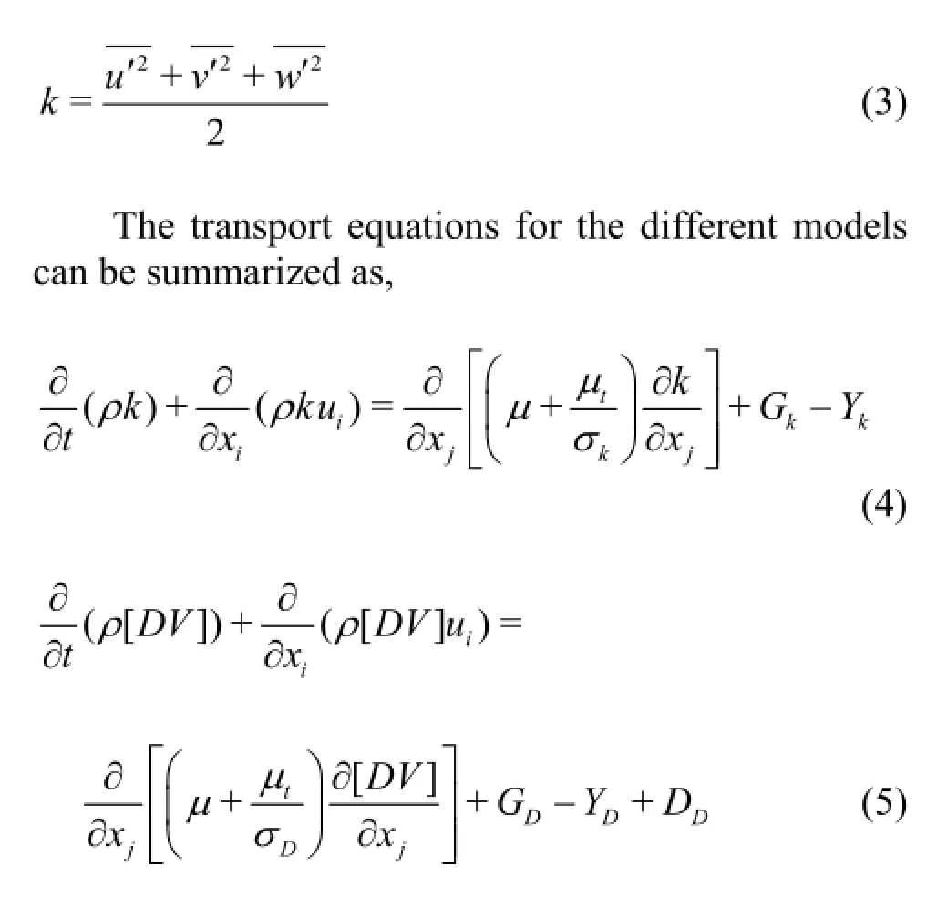
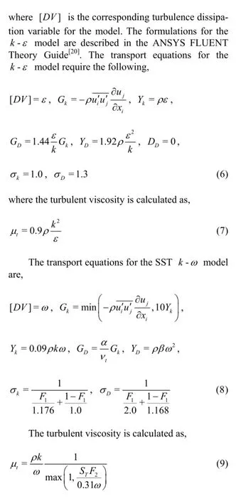
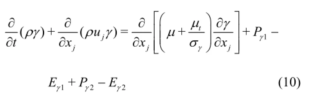
In these equations, not all the variables are constants as is the case for the -kεmodel. The transition SST model couples two additional transport equations with the SST -kωtransport equations. The first additional transport equation is for the intermittency,γ, defined as,

The onset of transition is controlled by,

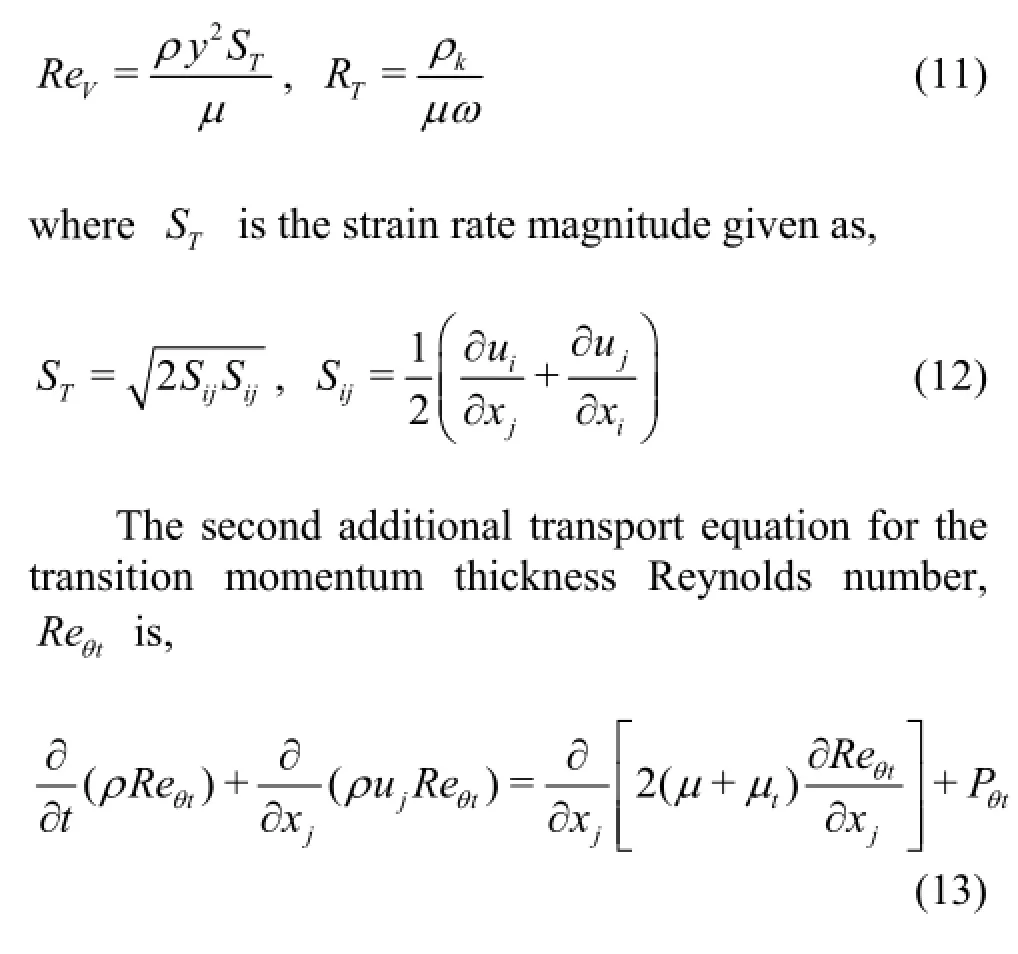
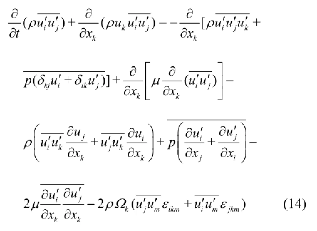
whereReθpis a proprietary empirical correlation for the transition onset andFθtis a function based on the boundary layer correlations. The transport equation for the RSM is,

1.2High performance computing

A third-order MUSCL scheme is applied for the momentum and turbulence solvers with the pressurevelocity coupled scheme. A convergence tolerance of 10-10is set for all simulations to ensure the iterative errors are much smaller than the grid errors such that the former can be neglected. Simulations are conducted using several local workstations and on University of Idahoʼs HPC computing resource, Big-STEM, using 8-12 core CPUʼs. Results are post-processed using Scilab-5.4.1 and Tecplot 360 2013.

1.3Iterative and statistical convergence

Statistical convergence of the running mean on the time history of the resistance establishes statistically stationary unsteady solutions[21]. Statistical convergence for the unsteady simulation is determined using the drag coefficient,DC, defined as,

The drag coefficient is monitored during the simulation. Data are collected once the drag coefficient oscillations around the mean value vary by only 1% of the mean value.

1.4Solution verification method

Solution verification is important to estimate the numerical errors and grid uncertainties of a CFD simulation. Numerical errors are due to the numerical solution of the mathematical equations. Aspects of the simulation that cause numerical errors include: discretization, artificial dissipation, incomplete iterative and grid convergence, and computer round-off. To determine numerical errors generally involves performing a sensitivity study by varying the mesh spacing and/or time step size to a smaller value and evaluating the solution differences. HereS1,S2,S3represent the fine, medium, and coarse grid solutions of any variable in the simulations, respectively. The relative percentage difference (δ%) between CFD results and correlation values, represented below asA, is calculated as,

The solution verification method in place is the factor of safety method[22,23]which requires the use of the following equations with the use of L2 norm for profiles[24],

where the grid uncertainty,UG, is presented as a percentage of the correlation value or value from the fine grid solution at the same streamwise location. A lower magnitude ofUGusually indicates a better quality of CFD results.

1.5Analysis method

However, the flow considered herein is unheated. Hence, the entropy generation occurs only due to the square of the gradients of the mean streamwise velocity. The integral over the boundary layer of the pointwise entropy generation rate provides the entropy generation rate per unit area,

The dissipation coefficient,Cd, is a dimensionless variable that represents the entropy generation rate per unit area. The correlation by McEligot and Walsh estimate the dissipation coefficient multiplied byReθas,

Both the displacement thickness and momentum thickness are integrated toδin place of the upper indefinite bound. Fluctuations in bypass transitional flows necessitate additional terms to the entropy generation equations used for laminar flow. These equations are outlined further by Walsh et al.[1].The dimensionless entropy generation rate per unit area for a transitional flow is calculated as,

whereu＇,v＇,w＇ are the velocity fluctuations in thex,yandzdirections, respectively. The dimensionless form of Eq.(27) is the dissipation coefficient,

Intermittency is a measure for determining the laminar, transition, and turbulent regions of the flow and is calculated as,

Fig.1 Mean velocity profile at inlet

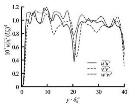
Fig.2 Reynolds normal stress profiles at inlet

2. Simulation design and verification

2.1Geometry and flow conditions

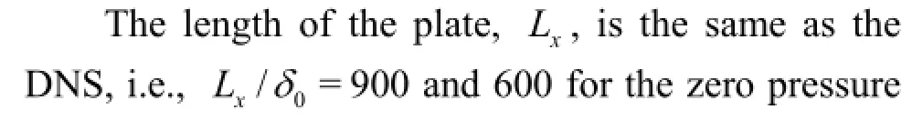
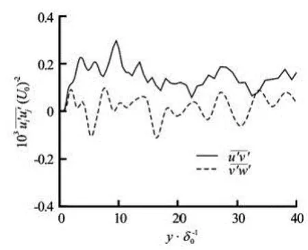
Fig.3 Reynolds shear stress profile at inlet

Fig.4 Geometry and mesh representation

Theεandωvalues at the inlet and for all models, are estimated using the equations from the ANSYS FLUENT Userʼs Guide[25]as,

While the Reynolds shear stresses are specified directly at the inlet for the RSM. The use of the inlet meanprofiles from DNS in the current study is more accurate boundary conditions compared to those applied by Ghasemi et al.[18]wherein the inlet boundary condition is specified with a constant turbulent intensity of 3% and a turbulent length scale equal to the boundary layer thickness.

2.2Mesh and simulation table

The mesh is created in Pointwise v17.0R1. The grid points in the streamwise direction are uniform and the grid points in the plate-normal direction are clustered near the plate surface, as shown in Fig.4. To assign more grid points toward the wall ensures that enough grid points exist within the boundary layer to capture the high velocity gradients in the boundary layer. A medium mesh and a coarse mesh were created for the solution verification study using a constant grid refinement ratio1/22. Figure 4 shows a schematic representation of the domain with an exaggerated curvature of top wall. The figure is a representation of an adverse pressure gradient geometry and mesh. The coordinate axis and boundaries are labeled.

A general overview of the different simulations performed in this study is contained in Table 1.2.3Solution verification

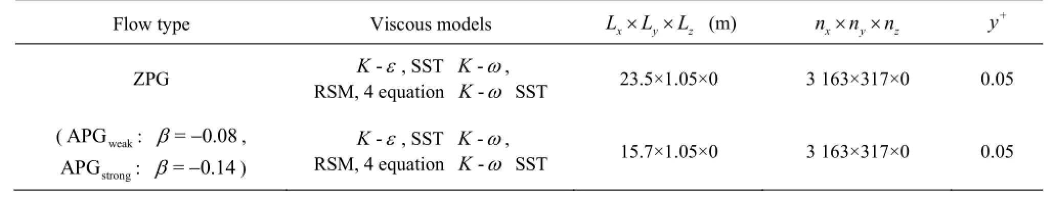
Table 1 Simulation design table

Table 2 Solution verification for bypass transitional boundary layer flow

The results from the solution verification study for thek-ωmodel are shown in Table 2. The distance to the asymptotic range (PG=1) is shorter forReθthanCf. Monotonic convergence is achieved. The grid uncertainty is below 1.6%S1for both variables. The solution verification study shows that the bypass transition results are independent of the grid resolution and thus all results are presented on the fine grid.

3. Results and discussion

The bypass transition simulation results are compared with the DNS results from Nolan and Zaki[17]. Additionaly, the ZPG results are compared to the CFD results by Ghasemi et al.[18]and APG results with Ghasemi et al.[19]. The current simulations employ a more accurate inlet conditions and much finer mesh than the simulations by Ghasemi et al. Thek,ω,z, profiles and Reynolds stress values are prescribed at the inlet, depending on the model in use, to match the conditions of the DNS simulation. Ghasemi et al. applied a velocity inlet boundary with a specified turbulent intensity of 3% and a turbulent length scale, whereas the mean velocity and turbulent structure profiles obtained from DNS[17]data are specified at the inlet in the current study. Additionally, this study also examines both CFD predictions for entropy generation rates compared to that post-processed from DNS results.

Fig.5 Reθversus Re1x/2

3.1Zero pressure gradient (ZPG)

Fig.6 Reθversus1/2xRe (detailed view near inlet)

Figure 7 and Fig.8 show how Cfand Cdvary with Re1x/2, respectively. The dissipation coefficient, Cd, provides a measure of the pointwise entropy generation rate, S＇＇＇ (in non-dimensional form), within the boundary layer for ZPG case as described earlier. The DNS data has a linear slope in the turbulent regime. The laminar region is the initial downward slope, the rise indicates the transition region, and the small oscillations downstream are within the fully turbulent region. Figure 7 also shows the analytical laminar and turbulent lines. Similar to the trends seen in Fig.5, the k-ε model and RSM transition to turbulent profile very close to the inlet and remain turbulent throughout the flow field.

Fig.7 Cfversus Re1x/2

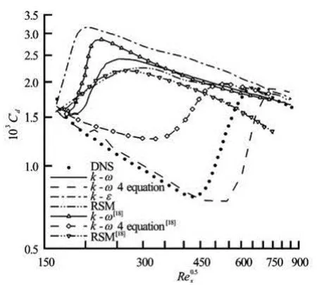
Fig.8 Cdversus Re1x/2

In Fig.7, the k-ε model shows an initial laminar profile near the inlet, similar to DNS, before transition occurs downstream. The k-ω model shows a laminar region until Re1x/2=215, where the onset of transition is predicted by the model. The k-ω model shows close agreement of predicted Cfto the DNS data from the inlet until the onset of transition and also in the turbulent region but transition occurs upstream compared to the k-ω 4 equation model and the DNS data. The k-ω 4 equation model shows better agreement with the DNS data for both Cdand Cf. The Cdand Cfpredicted by the k-ω 4 equation model is very accurate compared to the DNS data until the transitional point in DNS at Re1x/2=450. The model, however, over predicts the location of the onset of transition which occurs much later than DNS at Re1x/2=575.

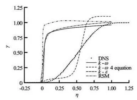
Fig.9 γ versus η

Fig.10 Cfversus Re1x/2for various RANS models for APGweak

Figure 9 shows that all turbulence models examined in this study predict transition onset (γ≤0.05) earlier than the DNS data. The k-ω, k-ε, and RSMʼs demonstrate very similar trends with steeper slopes than the k-ω 4 equation models. The k-ω 4 equation model is the closest to the DNS data in predicting the transition onset location but over-predicts γ by as much as 10% in the fully turbulent region. All models tend to predict a much steeper slope in the transition region compared to the much smoother slope in the DNS data.

3.2Adverse pressure gradient (APG)

The bypass transition simulation results for APG cases are also compared to the DNS results from Nolan and Zaki[17]and the CFD results by Ghasemi et al.[19]. The APG results are evaluated using the skinfriction coefficient,fC, and the approximate pointwise entropy generation rate, S＇＇＇.

3.2.1 APGweak: β=-0.08

The under prediction of Cfin the fully turbulent regime compared to Ghasemi et al.[19]is due to the differences in the inlet boundary conditions specified. Specifying a constant turbulent intensity of 3% and a specific length scale rather a mean profile for turbulent structures as in the simulations by Ghasemi et al. could result in over prediction of fully turbulent regime compared to the actual capabilities of each RANS model.

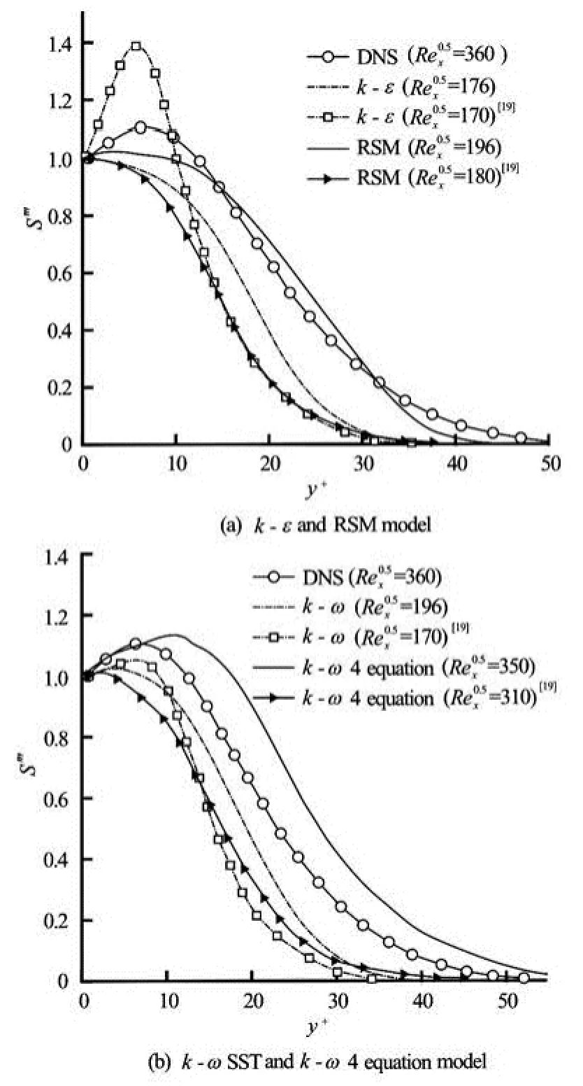
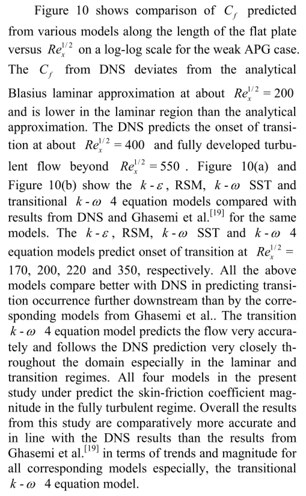
Fig.11 S＇＇＇ versus y+for various RANS models for APGweaknear location of transition shown by values of Re1x/2

Figure 11 shows the comparison of approximate point-wise entropy generation rates, S＇＇＇, as predicted by each model within the boundary layer plotted normal to the wall in terms of y+. Since different models predict varying locations of transition, the entropy generation rate (S＇＇＇) comparison is made at different locations along the flat plate for each model. These locations (indicated by Re1x/2values) are selected at a point near the onset of transition as predicted by each model.

Figure 11(a) shows the -kε and RSM model and Figure 11(b) shows the -kω SST and transitional -kω 4 equation models compared with results from DNS and Ghasemi. As seen from the figures the predictions from the current study are more accurate in terms of trends, magnitude and location than from Ghasemi for all corresponding models compared to DNS values. This is a direct result of better resolution within the boundary layer using more grid points near the wall and keeping y+＜1 at the first grid point away from the plate. The predictions from the k-ε, RSM and k-ω SST are considerably closer to DNS values than Ghasemi et al.. The transitional k-ω 4 equation model is the most accurate among all models although it slightly over-predicts the magnitude of S＇＇＇.

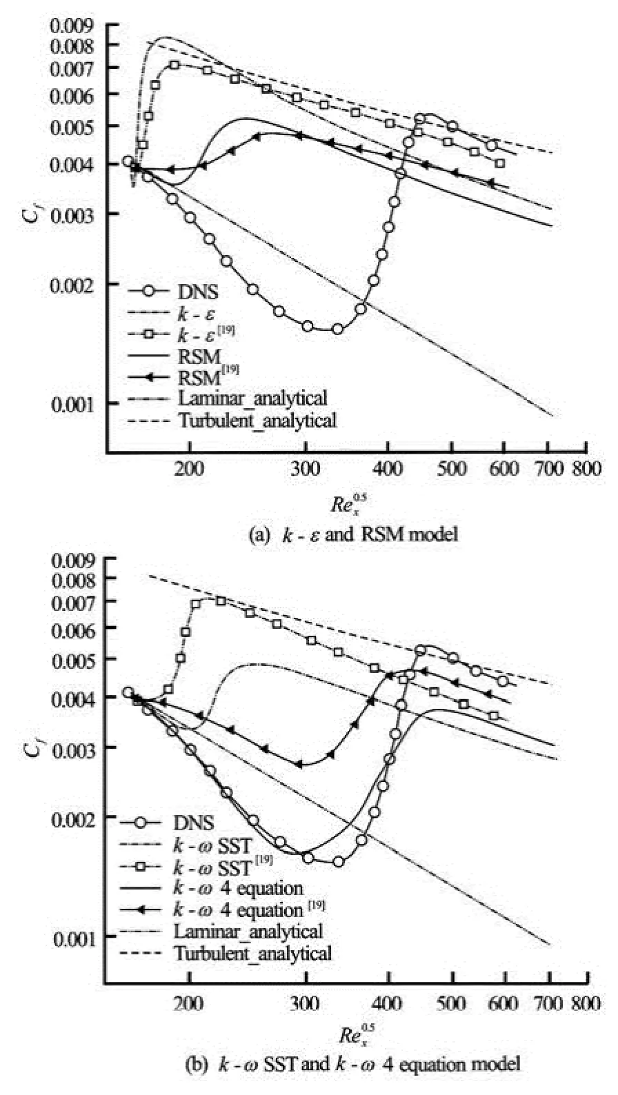
Fig.12 Cfversus Re1/2xfor various RANS models APGStrong

3.2.2 APGstrong: β=-0.14

小学语文教学不应该只局限于课本上几篇简单的文章和诗歌，老师应该多鼓励学生们进行课外的阅读来辅助语文学习，只要是文字优美的符合小学生认知规律和能力都可以鼓励学生进行广泛阅读，通过课外阅读他们也可以体会到文字的魅力也可以有效地提升学生们的语感，间接性的提高学生们的口语表达能力，同时也能为以后学生的写作打下坚实的阅读和写作基础。

Figure 12 shows the comparison of Cfpredicted from various models along the length of the flat plate versus Re1/2xon a log-log scale. The DNS[17]results show that Cfdeviates from the Blasius laminar approximation at approximately Re1x/2=180 and predicts a lower Cfvalue in the laminar region as seen in the previous APGweakcase.

The stronger adverse pressure gradient causes an earlier shift on predicted Cffrom the analytical app-roximation. The DNS predicts the onset of transition at about Re1x/2=330 and fully developed turbulent flow beyond Re1x/2=450. The Stronger APG also shows an increase the maximum magnitude of S＇＇＇from 1.1 in the APGweakcase to a value of 1.5.

Figure 12(a) show the k-ε and RSM model and Fig.12(b) shows the k-ω SST and transitional k-ω 4 eqation models. The k-ε, RSM, k-ω SST and k-ω 4 equation models predict onset of transition at=170, 195, 210 and 290, respectively. The k-ε model transitions to fully turbulent flow near the inlet for the current study as in the study by Ghasemi et al.. This may be a result of the stronger pressure gradient being imposed on the flow and thereby indicating the models incapability in handling strong adverse pressure gradients effectively. The RSM, k-ω SST and k-ω 4 equation models follow similar trends as seen in the APGweakcase with better comparison to DNS values than that by Ghasemi et al.[19].

Fig.13 S＇＇＇ versus y+for various RANS models APGStrong

Following the trend seen in previous results the models in current study under predict magnitude of Cfin the fully turbulent regime. Possible causes for such under prediction maybe as noted earlier in APGWeakresults.

Figure 13 shows the comparisons of predicted approximate point-wise entropy generation rate S＇＇＇within the boundary layer normal to the wall near the location of transition point in terms of y+. It is noteworthy that, since the k-ε model transitions near the inlet under the strong adverse pressure gradient, Fig.13(a) shows a turbulent profile of predicted entropy generation rate at Re1x/2=175 for this model. The RSM, k-ω SST and k-ω 4 equation models predict more accurate comparable profiles for S＇＇＇ near their transition location than the models by Ghasemi et al..

4. Conclusions and future work

In the future, the capability of using differentLES models to predict entropy generation rates for bypass transitional flows with and without streamwise pressure gradients will be evaluated. Sensitivity of LES models to grid resolution and time step size will be examined following the recent general framework for LES verification and validation[26,27]. The use of unsteady hydrodynamic instabilities in velocity and turbulent structure profiles at the inlet may lead to more accurate CFD predictions for bypass transitional boundary layer flows for both RANS and LES models.

Acknowledgements

This work was supported by the U.S. Department of Energy, Office of Science, Basic Energy Sciences, under Award # DE-SC0004751. The authors would also like to thank Dr. Tamer Zaki, Dr. Kevin Nolan, and Dr. Edmond Walsh for meaningful contributions.

[1] WALSH E. J., MCELIGOT D. M. and BRANDT L. et al. Entropy generation in a boundary layer transitioning under the influence of freestream turbulence[J]. Jour- nal of Fluids Engineering, 2011, 133(6): 061203.

[2] ZAKI T. A., DURBIN P. A. Mode interaction and the bypass route to transition[J]. Journal of Fluid Mecha- nics, 2005, 531(1): 85-111.

[3] MCELIGOT D. M., WALSH E. J. and LAURIEN E. et al. Entropy generation in the viscous parts of turbulent boundary layers[J]. Journal of Fluids Engineering, 2008, 130(6): 061205.

[4] SPALART P. R. Direct simulation of a turbulent boundary layer up to Reθ=1410[J]. Journal of Fluid Mechanics, 1988, 187(1): 61-98.

[5] SPALART P. R. Numerical study of sink-flow boundary layers[J]. Journal of Fluid Mechanics, 1986, 172(1): 307-328.

[6] ROTTA J. Turbulent boundary layers in incompressible flow[J]. Progress in Aerospace Sciences, 1962, 2(1): 1-95.

[7] MCELIGOT D. M., WALSH E. J. and LAURIEN E. et al. Entropy generation in the viscous layer of a turbulent channel flow[R]. Idaho National Laboratory (INL), 2006.

[8] ABE H., KAWAMURA H. and MATSUO Y. Direct numerical simulation of a fully developed turbulent channel flow with respect to the reynolds number dependence[J]. Journal of Fluids Engineering, 2001, 123(2): 382-393.

[9] KRAUSE E., OERTEL H. J. and SCHLICHTING H. Boundary-layer theory[M]. New York, USA: Springer, 2004.

[10] MCELIGOT D. M., NOLAN K. P. and WALSH E. J. Effects of pressure gradients on entropy generation in the viscous layers of turbulent wall flows[J]. International Journal of Heat and Mass Transfer, 2008, 51(5-6): 1104-1114.

[11] TSUKAHARA T., SEKI Y. and KAWAMURA H. et al. DNS of turbulent channel flow at very low Reynolds numbers[C]. Proceedings of the 4th International Symposium on Turbulence and Shear Flow Pheno- mena. Williamsburg, USA, 2005, 935-940.

[12] WALSH E. J., MCELIGOT D. M. A New correlation for entropy generation in low Reynolds number turbulent shear layers[J]. International Journal of Fluid Me- chanics Research, 2009, 36(6): 566-572.

[13] ABE H., KAWAMURA H. and MATSUO Y. Surface heat-flux fluctuations in a turbulent channel flow up to Reτ=1020 with Pr=0.025 and 0.71[J]. International Journal of Heat and Fluid Flow, 2004, 25(3): 404- 419.

[14] HOYAS S., JIMÉNEZ J. Scaling of the velocity fluctuations in turbulent channels up to Re=2003[J]. Physics of fluids, 2006, 18(1): 011702.

[15] SCHLATTER P., BRANDT L. and De LANGE H. et al. On streak breakdown in bypass transition[J]. Physics of fluids, 2008, 20(1): 101505.

[16] BRANDT L., SCHLATTER P. and HENNINGSON D. S. Transition in boundary layers subject to free-stream turbulence[J]. Journal of Fluid Mechanics, 2004, 517: 167-198.

[17] NOLAN K., ZAKI T. A. Conditional sampling of transitional boundary layers in pressure gradients[J]. Jour- nal of Fluid Mechanics, 2013, 728: 306-339.

[18] GHASEMI E., MCELIGOT D. and NOLAN K. et al. Entropy generation in a transitional boundary layer region under the influence of freestream turbulence using transitional RANS models and DNS[J]. International Communications in Heat and Mass Transfer, 2012, 41(1): 10-16.

[19] GHASEMI E., MCELIGOT D. M. and NOLAN K P. et al. Effects of adverse and favorable pressure gradients on entropy generation in a transitional boundary layer region under the influence of freestream turbulence[J]. International Journal of Heat and Mass Transfer, 2014, 77(1): 475-488.

[20] ANSYS. “FLUENT theory guide v14.0.0.”[R]. 2011.

[21] XING T., BHUSHAN S. and STERN F. Vortical and turbulent structures for KVLCC2 at drift angle 0, 12, and 30 degrees[J]. Ocean Engineering, 2012, 55(3): 23-43.

[22] XING T., STERN F. Closure to “Discussion of “Factors of safety for Richardson extrapolation”ʼ (2011, Journal of Fluids Engineering, 133, 115501)[J]. Journal of Fluids Engineering, 2011, 133(11): 115502.

[23] XING T., STERN F. Factors of safety for richardson extrapolation[J]. Journal of Fluids Engineering, 2010, 132(6): 061403.

[24] WILSON R. V., STERN F. and COLEMAN H. W. et al. Comprehensive approach to verification and validation of CFD simulations-Part 2: Application for rans simulation of a cargo/container ship[J]. Journal of Fluids Engineering, 2001, 123(4): 803-810.

[25] ANSYS. “FLUENT user guide v14.0.0.”[R]. 2011.

[26] XING T., GEORGE J. Quantitative verification and validation of large eddy simulations[C]. ASME 2014 Verification and Validation Symposium. Las Vegas, Nevada, USA, 2014.

[27] XING Tao. A general framework for verification and validation of large eddy simulations (keynote speaker)[C]. Proceedings of the 13th National Congress on Hydrodynamics and 26th Conference on Hydrodynamics. Qingdao, China, 2014, 40-58.

10.1016/S1001-6058(14)60075-5

* Biography: GEORGE Joseph (1986-), Male,

Master Candidate

XING Tao, E-mail: xing@uidaho.edu