LIU Shi-he (刘士和), XUE Jiao (薛娇), FAN Min (范敏)

State Key Laboratory of Water Resources and Hydropower Engineering Science, Wuhan University, Wuhan 430072, China

The calculation of mechanical energy loss for incompressible steady pipe flow of homogeneous fluid*

LIU Shi-he (刘士和), XUE Jiao (薛娇), FAN Min (范敏)

State Key Laboratory of Water Resources and Hydropower Engineering Science, Wuhan University, Wuhan 430072, China

(Received June 4, 2013, Revised October 25, 2013)

The calculation of the mechanical energy loss is one of the fundamental problems in the field of Hydraulics and Engineering Fluid Mechanics. However, for a non-uniform flow the relation between the mechanical energy loss in a volume of fluid and the kinematical and dynamical characteristics of the flow field is not clearly established. In this paper a new mechanical energy equation for the incompressible steady non-uniform pipe flow of homogeneous fluid is derived, which includes the variation of the mean turbulent kinetic energy, and the formula for the calculation of the mechanical energy transformation loss for the non-uniform flow between two cross sections is obtained based on this equation. This formula can be simplified to the Darcy-Weisbach formula for the uniform flow as widely used in Hydraulics. Furthermore, the contributions of the mechanical energy loss relative to the time averaged velocity gradient and the dissipation of the turbulent kinetic energy in the turbulent uniform pipe flow are discussed, and the contributions of the mechanical energy loss in the viscous sublayer, the buffer layer and the region above the buffer layer for the turbulent uniform flow are also analyzed.

mechanical energy loss, energy equation, pipe flow

Introduction

The mechanical energy is the sum of the potential energy and the kinetic energy. The calculation of the mechanical energy loss between two sections along the main flow direction is an important problem in practical engineering, as well as an important research topic in Engineering Fluid Mechanics and Hydraulics.

In the field of Hydraulics, the mechanical energy loss is usually called the resistance loss, which is divided into the friction loss and the local loss, and the resistance coefficient is mainly determined by experiments. For example, Reynolds carried out experiments to study the differences of the resistance coefficients in laminar and turbulent pipe flows, Nikuradse conducted experiments for flows in artificially roughened pipes and obtained the variation of the resistance loss against the Reynolds number and the relative roughness of the pipe wall. Many studies of the resistance loss were based on these two fundamental studies[1-5].

In the field of Fluid Mechanics, many studies focused on the mechanisms of turbulent flow[6-9], flow stability[10]and the related spatial or temporal distributions of the flow quantities. With regards to pipe flows, Samanta et al.[11]carried out the experimental investigation of the laminar turbulent intermittency in pipe flows, Liu et al.[12]studied the velocity distributions in the transition region of pipes with Particle Image Velocimetry (PIV), Van Doorne and Westerweel[13]investigated the flow characteristics of laminar, transitional and turbulent pipe flows by using Stereoscopic Particle Image Velocimetry (SPIV), Genç et al[14]studied the Reynolds stresses in a swirling turbulent pipe flow with Laser-Doppler Anemometer (LDA), Wagner et al.[15], Wu and Moin[16]studied the turbulent pipe flow by Direct Numerical Simulation (DNS).

However, the relation between the mechanical energy loss in the volume between two cross sections and the kinematical and dynamical characteristics of the flow field was not addressed for a non-uniform flow in previous studies. This paper derives a new mechanical energy equation for incompressible steady non-uniform pipe flows of homogeneous fluid, including the variation of the mean turbulent kinetic energy,and the theoretical results for uniform flows are used for comparison. Furthermore, the contributions of the mechanical energy loss are analyzed relative to the time averaged velocity gradient and the dissipation of the turbulent kinetic energy in a uniform flow, in different regions, especially in the radial direction.

1. Formulation of the mechanical energy equation

Considering the flow of homogeneous incompressible fluid in the gravitational field, the second order tensor of the surface force[6]ijTcan be expressed as

whereρis the fluid density,fiis the mass force per unit volume anduiis the velocity components. Decompose the surface force tensor asTij=-pδij+τij, wherepis the pressure,τij=2μsijis the viscous stress andsijis the rate of deformation. For an incompressible steady flow of homogeneous fluid in the gravitational field (letx3be the vertical coordinate), we have

In Eq.(2),gx3+p/ρ+ujuj/2 is the mechanical energy, therefore this equation is the differential form of the mechanical energy equation for an incompressible steady flow of homogeneous fluid in the gravitational field, the integral form of the corresponding mechanical energy equation for a steady pipe flow in laminar and turbulent states (corresponding to the statistical quantities in ensemble average) will be discussed afterwards based on this equation.

1.1Laminar flow

Consider a control volumeVas shown in Fig.1, where the entire surface is expressed asA, including two cross-sections1A,2Aat the upstream and the downstream with distanceLand the pipe wall, and the flows in this volume are gradually varied. Integrating Eq.(2) overV, and using the Gaussian Theorem to transform the volume integral into the surface integral for the left hand side and the first term on the right hand side, then

wherejnis the component of the unit normal vector of the surfaceA. For a simple laminar shear flow, the potential energygx3+p/ρ(which is called the piezometric head in Hydraulics) on eitherA1orA2are constant since the flows across these sections are the gradually varied flows[6]. Noting that the velocity on the pipe wall is zero we have

whereAis the cross-sectional area andUis the mean velocity at a section, andzis substituted forx3for the vertical coordinate to conform with the symbols used in Hydraulics and Engineering Fluid Mechanics. The indexes 1 and 2 are used to represent the corresponding quantities at cross sectionsA1andA2. Define the kinetic energy correction coefficientsα1andα2such that

and usewhto represent the mechanical energy transformation (the second and third terms on the right hand side of Eq.(5)) and the loss (the first terms on the right hand side of Eq.(5)) per unit weight in unit time, i.e.,

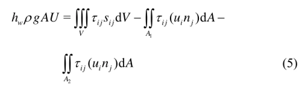
the total mechanical energy equation Eq.(3) for a laminar flow then becomes

It can be seen from Eq.(6) that a part of the mechanical energy is consumed owing to the viscous effect when the fluid flows from the cross section1Ato 2A.

Fig.1 Sketch of pipe flow

If the shape and the size of the cross sections1Aand2Aare identical, andijτ,iuhave the same distributions on them, we have

i.e., there would be no mechanical energy transformation while the fluid flows from cross section1AtoA2. In this case the mechanical energy loss becomes

Furthermore, if the flow included between the cross sections1Aand2Ais uniform, the mechanical energy loss can be simplified as

1.2Turbulent flow

Apply the Reynolds decomposition to Eq.(2), and then take the ensemble average. For a steady turbulent flow in the sense of ensemble averaged quantities we have

therefore, Eq.(8) can be obtained by taking ensemble average

Integrating Eq.(8) over the control volumeV, and using the Gauss Theorem to transform the volume integral into the surface integral for the left hand side and the second term on the right hand side, we have

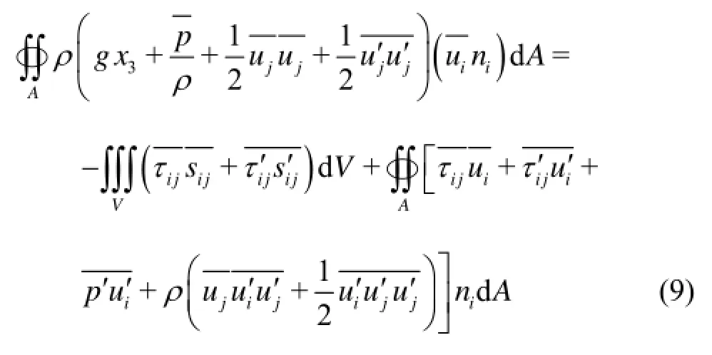
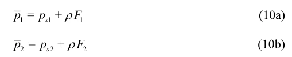
For a non-circular turbulent pipe flow, the hydrostatic assumption (the hydrodynamic pressure is equal to the hydrostatic pressure at the cross section of gradually varied flow) would not be hold, strictly speaking, owing to the non-homogeneity of the Reynolds stresses and the secondary flow at the cross section. Usingspto represent the hydrostatic pressure such thatgx3+ps/ρ=C, and usingρF1andρF2to represent the deviations between the hydrodynamic pressuresp1andp2and the hydrostatic pressuresps1and 2spat the cross-sections 1Aand 2A, by using the method of Green function[6], we have

Similar to the discussions in Section 1.1, define themean kinetic energy correction coefficients1α,2αand the mean turbulent energy correction coefficients 1βand2βat the cross-sections1Aand2Asuch that

and usewhto represent the transformation(the second term on the right hand side of Eq.(12)) and loss (the first terms on the right hand side of Eq.(12)) of the mechanical energy. Equation (9) can be simplified by using the no-slip condition on the pipe wall such that

Equation (11) is the integral form of the mechanical energy equation for the incompressible steady nonuniform pipe flow of homogeneous fluid, which includes the variation of the mean turbulent kinetic energy from1Ato2A. In Eq.(11)

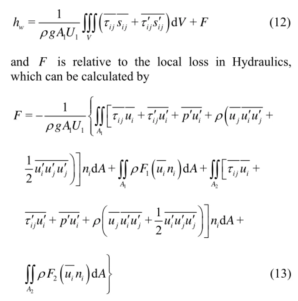
Furthermore, if the flow between the cross sections1Aand2Ais uniform (for example, the flow in a long and straight pipe), the mechanical energy loss can be further simplified as

2. Mechanical energy loss for steady uniform laminar flow in a circular pipe

For the steady uniform laminar flow in a circular pipe the longitudinal velocityzuonly changes in the radial directionrsuch that[6]

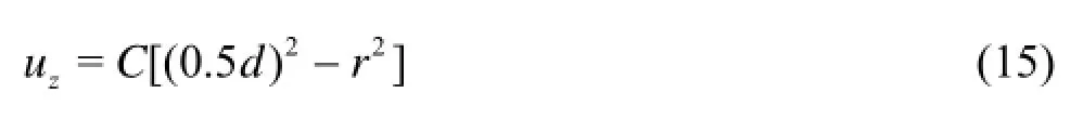
wheredis the diameter of the circular pipe andCis a constant related to the mean pressure gradient in thelongitudinal direction. Substituting Eq.(15) into Eq.(7b) the following equation can be obtained finally after some simplifications

Equation (16) is the same as the Darcy-Weisbach formula for the resistance loss of a steady uniform laminar flow in a circular pipe in Hydraulics, and the resistance coefficientλ=64/Red, whereRed=U1d/νis the Reynolds number.

3. Mechanical energy loss for uniform turbulent flow in a circular pipe

For the uniform turbulent flow in a circular pipe the longitudinal velocityzualso only changes in the radial direction, using the condition of the axial symmetry Eq.(14b) can be rewritten as It can be seen from Eq.(17) that the mechanical energy loss has two parts, both from the fluid viscosity for the uniform turbulent flow in a circular pipe, the former is related to the time averaged velocity gradient and the latter is related to the dissipation of the turbulent kinetic energy. For the uniform turbulent flow in a circular pipe, the total dissipation of the turbulent energy is equal to the total generation of the turbulent energy at section1A, i.e.,

Therefore Eq.(17) can be simplified considering that

for the uniform turbulent flow in a circular pipe such that whereu*is the shear velocity. Defining the coefficient for the mechanical energy loss asλ=8(u*/U1)2, Eq.(19) can be simplified further as

Equation (20) is the same as the Darcy-Weisbach formula for the resistance loss for the steady uniform turbulent flow in a circular pipe in Hydraulics.

Now we discuss the compositions of the mechanical energy loss based on Eq.(17). From Eq.(20) and Eq.(17)λcan be expressed as

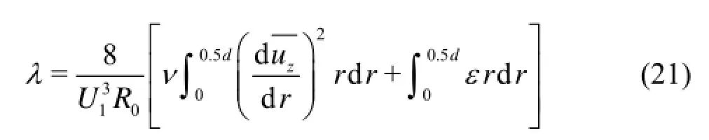
Using 1λand2λto represent the contributions to the coefficients of the mechanical energy loss relative to the time averaged velocity gradient and the dissipation of the turbulent kinetic energy, respectively, we have

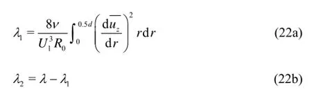
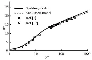
Fig.2 Comparison of theoretical velocity distribution with experimental data

Fig.3 Variation of1/λλand2/λλwithdRe

Fig.4 Contributions of viscous sublayer, buffer layer and the region above buffer layer to the mechanical energy loss

In the radial direction, the uniform turbulent flow in a circular pipe can be divided into a viscous sublayer (r∈(0.5d-5ν/u*～0.5d)), a buffer layer (r∈(0.5d-30ν/u*～0.5d-5ν/u*)), and the region above the buffer layer which contains the logarithmic region[6,17]. The contributions of the above three regions to the mechanical energy loss are calculated based on the time averaged velocity distributions relative to the Van Driest model and the Spalding formula, as shown in Fig.4. It can be seen that: (1) whendReis less than 2.5×104, the contributions of the above three regions to the mechanical energy loss are in the following order: buffer layer＞viscous sublayer＞the region above the buffer layer. (2) whendReis larger than 2.5×104and less than 1.3×105, the contributions of the above three regions to the mechanical energy loss are in the following order: buffer layer＞the region above the buffer layer＞viscous sublayer. (3) whendReis larger than 1.3×105, the contributions of the above three regions to the mechanical energy loss are in the following order: the region above the buffer layer＞buffer layer＞viscous sublayer.

4. Conclusions

(1) A new energy equation for incompressible steady non-uniform pipe flow of homogeneous fluid is derived, which includes the variation of the mean turbulent kinetic energy, and the formula for the calculation of the transformation and loss of the mechanical energy for the non-uniform flow between two cross sections is obtained based on this equation. This formula can be simplified to the Darcy-Weisbach formula widely used in Hydraulics for uniform flows.

(2) The mechanical energy loss of a turbulent flow is resulted from the fluid viscosity in a circular pipe and can be divided into two parts for a uniform flow, the first is related to the time averaged velocity gradient, and the other is related to the dissipation of the turbulent kinetic energy. The former decreases with the increase of the Reynolds number, and the latter increases with the increase of the Reynolds number. When the Reynolds number is larger than 3×104, the contribution from the term related to the dissipation of the turbulent kinetic energy is dominant.

(3) In the radial direction, the uniform turbulent flow in a circular pipe can be divided into the viscous sublayer, the buffer layer and the region above the buffer layer. With the increase of the Reynolds number, the contributions of the mechanical energy loss in the buffer layer and the viscous sublayer decrease, while the contribution from the region above the buffer layer increases. When the Reynolds number is larger than 1.3×105, the contribution of the mechanical energy loss in the region above the buffer layer becomes dominant.

[1] MCKEON B. J., ZAGAROLA M. V. and SMITS A. J. A new friction factor relationship for fully developed pipe flow[J].Journal of Fluid Mechanics,2005, 538: 429-443.

[2] SHOCKLING M. A., ALLEN J. J. and SMITS A. J.Roughness effects in turbulent pipe flow[J].Journal of Fluid Mechanics,2006, 564: 267-285.

[3] FADARE D. A., OFIDHE U. I. Artificial neural network model for prediction of friction factor in pipe flow[J].Journal of Applied Sciences Research,2009, 5(6): 662-670.

[4] YANG S. Q., HAN Y. and DHARMASIRI N. Flow resistance over fixed roughness elements[J].Journal of Hydraulic Research,2011, 49(2): 257-262.

[5] YOON J. I., SUNG J. and LEE M. H. Velocity profiles and friction coefficients in circular open channels[J].Journal of Hydraulic Research,2012, 50(3): 304-311.

[6] ZHANG Zhao-shun, CUI Gui-xiang.Fluid mechanics[M]. Second Edition, Beijing, China: Tsinghua University Press, 2006(in Chinese).

[7] MCKEON B. J., LI J. and JIANG W. et al. Further observations on the mean velocity distribution in fully developed pipe flow[J].Journal of Fluid Mechanics,2004, 501: 135-147.

[8] SAKAKIBARA J., MACHIDA N. Measurement of turbulent flow upstream and downstream of a circular pipe bend[J].Physics of Fluids,2012, 24(4): 041702.

[9] HULTMARK M., BAILEY S. C. C. and SMITS A. J. Scaling of near-wall turbulence in pipe flow[J].Journal of Fluid Mechanics,2010, 649: 103-113.

[10] WANG Xin-jun, LUO Ji-sheng and ZHOU Heng. Mechanism of breakdown process of the laminar-turbulent transition in plane channel flow[J].Science in China, Series G: Physics, Mechanics and Astronomy,2005, 35(1): 71-78(in Chinese).

[11] SAMANTA D., De LOZAR A. and HOF B. Experimental investigation of laminar turbulent intermittency in pipe flow[J].Journal of Fluid Mechanics,2011, 681: 193-204.

[12] LIU Yong-hui, DU Guang-sheng and LIU Li-ping et al. Experimental study of velocity distributions in the transition region of pipes[J].Journal of Hydrodynamics,2011, 23(5): 643-648.

[13] Van DOORNE C. W. H., WESTERWEEL J. Measurement of laminar, transitional and turbulent pipe flow using stereoscopic-PIV[J].Experiments in Fluids,2007, 42(2): 259-279.

[14] GENÇ B. Z., ERTUNÇ Ö. and JOVANOVIĆ J. et al. LDA measurements of Reynolds stresses in a swirling turbulent pipe flow[C].Proceedings of 12th EUROMECH European Turbulence Conference.Marburg, Germany, 2009, 132: 617-620.

[15] WAGNER C., HUTTL T. J. and FRIEDRICH R. Low Reynolds number effects derived from direct numerical simulations of turbulent pipe flow[J].Computers and Fluids.2001, 30(5): 581-590.

[16] WU X., MOIN P. A direct numerical simulation study on the mean velocity characteristics in turbulent pipe flow[J].Journal of Fluid Mechanics,2008, 608: 81-112.

[17] LIU Shi-he, LIU Jiang and LUO Qiu-shi et al.Engineering turbulence[M]. Beijing, China: Science Press, 2011(in Chinese).

10.1016/S1001-6058(13)60440-0

* Biography: LIU Shi-he (1962-), Male, Ph. D., Professor