Yi-Zi Cheng(承亦梓), Fu-Hong Min(闵富红), Zhi Rui(芮智), and Lei Zhang(张雷)

School of Electrical and Automation Engineering,Nanjing Normal University,Nanjing 210023,China

Keywords: memristive circuit,chaos,multistability,FPGA implementation

1. Introduction

Memristor,the 4th basic circuit element,[1]which reveals the relationship between flux and charge, has great application potentials in the fields of neural network,[2]nonlinear circuit design,[3]image encryption,[4]etc. In recent years, various novel memristor-based circuits were widely built, and the complex dynamical behaviors of such memristive systems have been also studied. For example, a Duffing oscillator with memristor was experimentally realized in Ref. [5],and a Chua’s circuit with memristor, which shows extreme multistability and other complex dynamics, was proposed in Ref. [6]. In Ref. [7], a discrete memristor model was defined and applied to H´enon map. An Sr0.95Ba0.05TiO3(SBT)memristor is a new kind of physical memristor, and the complex behaviors of memristive circuit based on SBT was studied in Ref. [8]. A variety of autonomous or non-autonomous oscillators based on memristors expanded the research areas for these nonlinear systems.[9–11]Compared with the conventional chaotic circuits,[12]the memristor-based circuits can easily procduce diverse nonlinear motions,such as self-excited chaotic behaviors,[13]hidden attractors,[14]hyperchaos,[15]and anti-monotonic properties.[16]Because the memristive circuit is sensitive to initial values, the multistability, a typical behavior of such circuits, has become a research hotspot in recent years. The multistability in circuits with single or multiple memristors has been reported by a large number of researches.[17–21]For example, the serial-parallel memristor was introduced into the Chua’s circuit, and the influence of memristor polarity and series-parallel structure on mutistability phenomenon was explored and concluded.[2]The memristive Chua’s circuit based on active band-pass filter (BPF)was studied,in which the stable distribution of the equilibrium points was divided to confirm the trace of memristive circuit starting from different initial states.[21]And then,the extreme multistability of infinite coexistence attractors was observed,which provides the guidance for further exploring the relationship between the equilibrium points and the multistability.

To make in depth analysis of the multistability, a new modeling method called state variable mapping (SVM) was proposed.[22]However, the SVM has its disadvantages: it is suitable only for the normalized state equation and those memristive systems with only simple nonlinear terms. To improve SVM, Chenet al.proposed a method of combining the incremental integral change with linear state variable,[23]which was named hybrid state variable incremental integral(HSVII).As the dimensionality reduction methods mentioned above still cannot directly simplify the model, in the light of flux–charge analysis method(FCAM)[24]which offers an effective way to analyze the infinite many dynamics caused by memristor, a dimensionality reduction analysis was carried out in the memeristive circuits in Ref.[25]. However,because of the complexity of the equation derivation and state variable selection, the application of FCAM in memristive systems has rarely been reported.

In this paper, a heterogeneous DMC with two different memristors, based on Chua’s circuit, is constructed, and its nonlinear dynamical behaviors are investigated from multiple perspectives. This DMC can be used for encrypting an image.The rest of this paper is organized as follows. In Section 2,the DMC schematics are presented, and their mathematical models in the voltage–current domains and the flux–charge domains are established respectively. In Section 3, the symmetrical bifurcation and the parameter mappings with specific parameters are discussed by the 5th-order model(5OM)in the volt–ampere domain. Subsequently in Section 4, the dimensionality reduction model, 3rd-order model (3OM) in flux–charge domain,is derived by FCAM,and its hardware circuit is realized through field-programmable gate array (FPGA).Then,the multistability is illustrated through attraction basins and phase diagrams in 3OM and 5OM.Finally,some conclusions are drawn in Section 6.

2. Circuit modeling

In this section, a memristive circuit with two different memristors is proposed based on Chua’s circuit. The voltage–ampere model of heterogeneous dual memristive circuit is derived by Kirchhoff’s law and the volt–ampere relationship,and the flux–charge model is subsequently obtained through flux–charge analysis method to make it more controllable.

2.1. Voltage–ampere model

The heterogeneous DMC is constructed based on memristive Chua’s circuit[26]as shown in Fig. 1, where the circuit consists of two capacitorsC1andC2, an inductorL, a linear negative conductance-G, a third-order nonlinear flux–controlled memristorW, and a charge-controlled memristorMdescribed by absolute value. For the rationality of the mathematical model,the flux–controlled memristorW(ϕ)and the capacitorC1are connected in parallel, while the chargecontrolled memristorM(q)and the inductorLare in series.

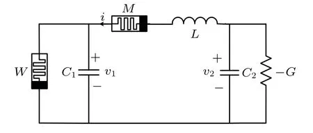
Fig.1. Heterogeneous DMC.

According to Kirchhoff’s law and the volt–ampere relationship, the state equation of the DMC can be derived into five first-order differential equations:

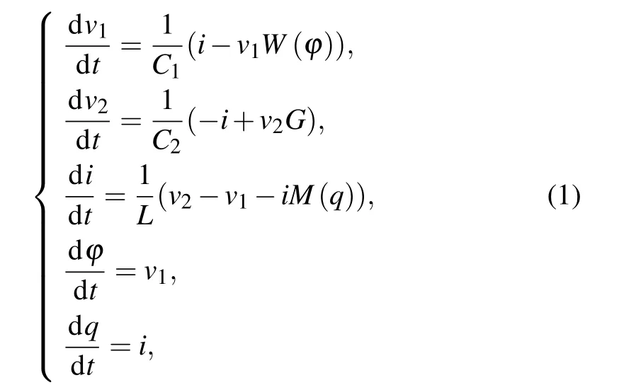
where the flux-controlled memristor is described asW(ϕ)=a+3bϕ2,the charge-controlled memristorM(q)=−c+d|q|,v1andv2represent the voltage of capacitorC1andC2,ithe current through the parallel branch of the charge-controlled memristor and the inductanceL,ϕthe internal flux of the cubic memristor,qthe internal charge of the quadratic memristor. Assumingv1=x,v2=y,i=z,ϕ=w,q=v,1/C1=α,1/C2=β,1/L=η,G=γ,we can obtain 5OM from Eq.(1)as follows:

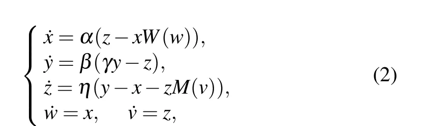
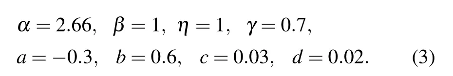
whereW(w)=a+3bw2andM(v)=−c+d|v|. For convenience,the system parameters are taken as

2.2. Flux–charge model

Through the flux–charge method, the increment of flux and charge from 0 totare defined asϕ(t;0)=ϕ(t)−ϕ(0)andq(t;0) =q(t)−q(0), respectively, whereϕ(0,0) = 0 andq(0,0)=0, the flux increments areϕM1(t;0),ϕM2(t;0),ϕC1(t;0),ϕC2(t;0),ϕL(t;0), andϕG(t;0). The charge increments areqM1(t;0),qM2(t;0),qC1(t;0),qC2(t;0),qL(t;0),andqG(t;0),and the reference directions are shown in Fig.2.

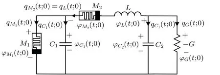
Fig.2. DMC with reference directions.

where the constitutive relationships of the elements can be obtained as follows:

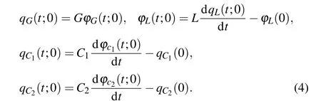
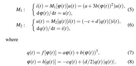
The initial values of the above elements are expressed asqC1(0) =C1uC1(0),qC2(0) =C2uC2(0),ϕL(0) =LiL(0),anduC1(0),uC2(0),iL(0) are equivalent to the initial values of the first three equations in Eq. (1). The model of fluxcontrolled memristor can thus be expressed asqM1(t;0) =f[ϕM1(t;0)+ϕM1(0)]−qM1(0), and the charge-controlled memristorϕM2(t;0) =h[qM2(t;0)+qM2(0)]−ϕM2(0), in whichqM1(0)=f[ϕM1(0)],ϕM2(0)=h[qM2(0)]. According to the actual circuit, the mathematical model of two memristors can be described as

Here,we seta=−0.3,b=0.6,c=0.03,andd=0.02.

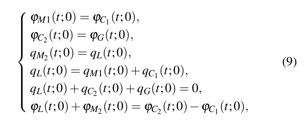
According to Kirchhoff’s law and the circuit model in Fig.2,it follows that

and the third-order differential equation

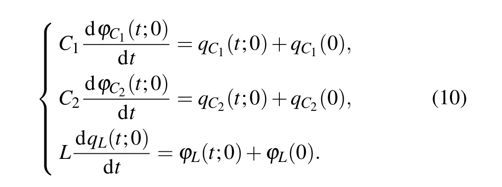
Substituting Eq.(9)into Eq.(10),we obtain in the flux–charge domain

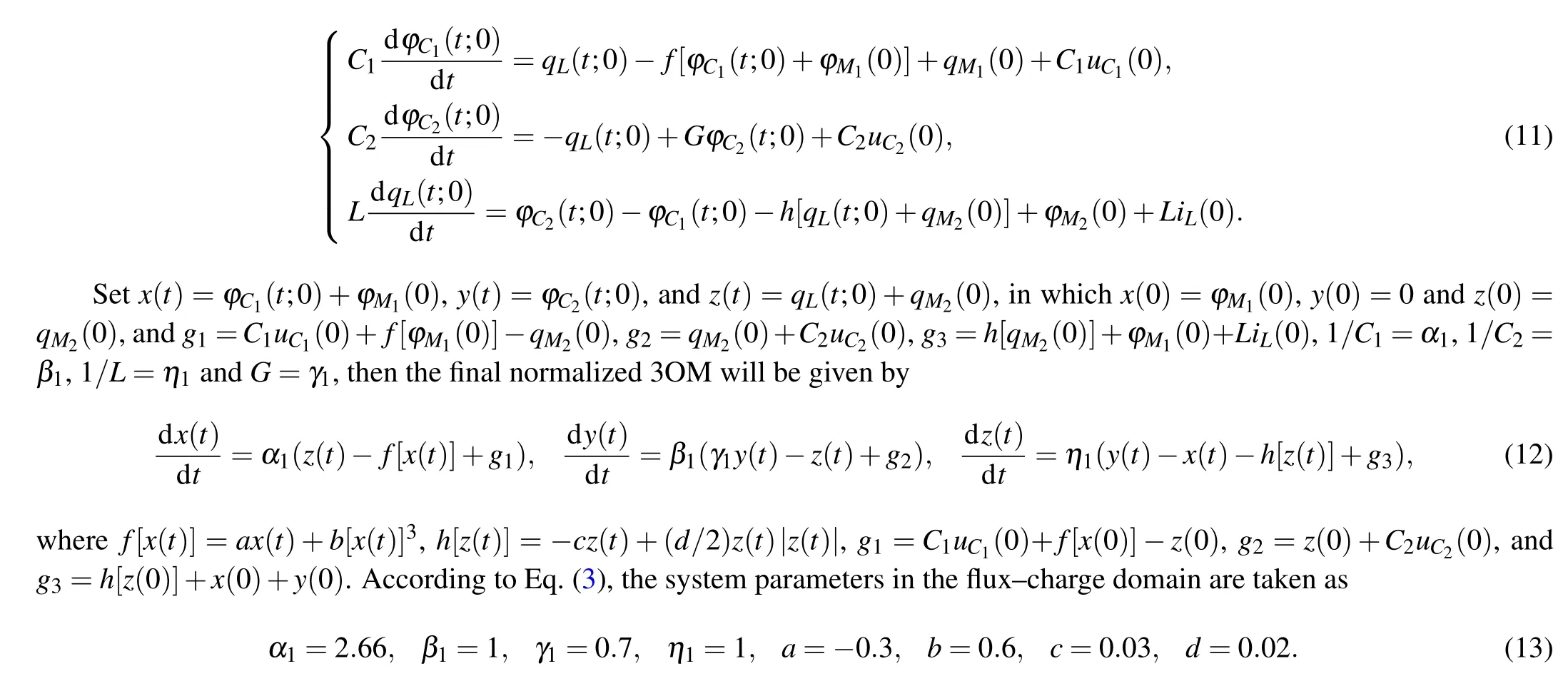
Compared with the 5OM, the 3OM converts the initial values into the system parameters,thereby improving the controllability of the circuit.

3. Symmetry sensitive to parameters

In this section,the symmetric dynamical behavior which depends on the system parameters is analyzed. Firstly, based on the volt–ampere model (2), the symmetric coexistence bifurcation behaviors under special conditions are studied.Then, aiming at the dimensionality reduction model(12), the motions with corresponding parameters are simulated,and the differences between the above two models are compared.

3.1. Symmetry in voltage–current domain

For the parameters in Eq. (3) and the initial conditions(±10−9,0,0,0,0),the bifurcation diagrams and Lyapunov exponent spectrumsversus γandηare calculated and depicted in Fig.3,where the blue represents the coexisting bifurcation diagram with (10−9,0,0,0,0), red denotes the coexisting bifurcation diagram with(−10−9,0,0,0,0),two superposed bifurcation trajectories ofxmaxcan be observed. As the variation trend of Lyapunov exponent spectrums under two opposite initial conditions are almost the same,only the Lyapunov exponent spectrums at positive initial condition are exhibited in Fig.3.

As can be seen from Fig.3,there are four symmetric motions, that is the following: ‘SP (stable point)’, ‘period(periodic state)’,‘CM(complex motion)’,and‘LP(large period)’.Forγincreasing in Fig. 3(a) andγ ∈(0.45,0.85), the system moves from SP to period, then to CM through perioddoubling bifurcation, and finally jumps to LP. Forηincreasing in Fig.3(b)andη ∈(0.65,1.95),the motion is exactly the opposite, starting from LP, then moving into CM and entering into period by reverse period-doubling bifurcation,finally dropping to SP. It should be noted that in the CM area, there appears mainly chaos with different periodic windows in the middle. Although the phase trajectories of the conventional period-1 and the large period are all limit cycles, while their Lyapunov exponents are different. When the large period appears,the minimum Lyapunov exponent will suddenly drop to an abnormally small value. In order to distinguish it between“period”and“LP”,the minimum Lyapunov exponent is used as a criterion.

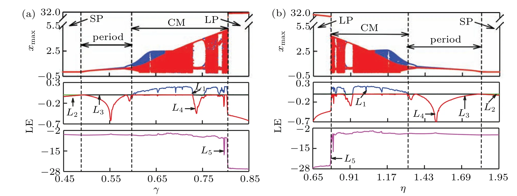
Fig.3. Bifurcation and Lyapunov exponent spectrum versus(a)γ and(b)η.

To intuitively show the distribution characteristics of the dynamical behaviors for varying parametersγandη, the parameter mappings (γ,α) and (η,α) are depicted respectively in Fig. 4, where four colors are used to mark four motions: ‘blue-SP’, ‘orange-period’, ‘purple-CM’, and ‘yellow-LP’.From Fig.4,we can see that the symmetric characteristic still exist within the attraction basins,and it is not affected by other parameters. The whole evolution of “SP–period–CM–LP”, in positive or reverse order, can be fully presented for 1.4≤α ≤6. Ifαis less than 1.4,no matter how other parameters are changed,the circuit always goes through two states,SP and period,in which the system is extremely stable. Phase diagrams of each motion are given in Fig. 5 withα=2.66 and(10−9,0,0,0,0)as verification. When the specific chaotic signals need to be used,it is necessary to avoid fixing the parameter range within this range. It can been seen thatγandηhave good symmetry, for theGand 1/Lhave opposite trends in circuit evolution while other parameters have little effect on the symmetry.

Fig.4. Parameter mappings with(10−9,0,0,0,0)on(a)γ–α plane and(b)η–α plane.

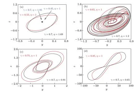
Fig.5. Coexisting attractors with α =2.66 and(10−9,0,0,0,0).

3.2. Symmetry in flux–charge domain

After the dimensionality reduction by FCAM, the initial values are converted into the system parameters in flux–charge model(12), which can make the in-depth analysis of the heterogeneous dual memristive circuit. The original system (2)has symmetrical characteristics,which should not be changed by the dimensionality reduction model(12). To validate this,the bifurcation trajectory and Lyapunov exponent spectrums of 3OM are calculated and illustrated in Figs. 6(a) and 6(b),

where the initial condition is (0,0,0), and the parameters are from Eq.(13).

From Fig.6,we know that the diagrams,such as symmetric bifurcation and four motions,look similar to those in Fig.3,which means that Eq. (12) is consistent with system (1). Forγ1∈(0.45,0.5),g1=±10−9, andg2=g3=0, as shown in Fig.6(a),the corresponding maximum Lyapunov exponentL1is less than zero,and the system is in the stable state. With increasingγ1∈(0.5,0.85), the system enters into the period 1,then changes to period 2 through the period-doubling bifurcation,subsequently moves into complex motion through saddle junction bifurcation,in which several periodic windows exist,finally,suddenly jumps into a large period withL1returning to zero,andL2showing a steep drop. However,forηincreasing,η1∈(0.65,1.95), the movement trend of Fig. 6(b) is almost opposite to that of Fig.6(a).The system first moves from LP to chaos,and then enters into multi-period from the saddle junction bifurcation. Finally,it goes into period 1 through reverse period-doubling bifurcation and then remains stable.

Comparing with the above analysis, it can be seen that the five-dimensional model in thev–idomain has been transformed into a three-dimensional model in theϕ–qdomain via FCAM.Although the system dimension decreases and the mathematical model changes,the dynamical behavior with the corresponding parameters does not change, and the special symmetric coexistence bifurcation still exists.

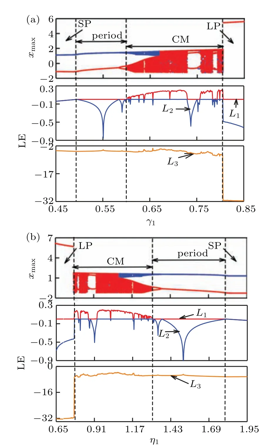
Fig. 6. Bifurcation diagrams and Lyapunov exponent spectra for (a) γ1 ∈(0.45, 0.85)and(b)η1 ∈(0.65, 1.95).

4. Multistability sensitive to initial conditions

In this section, the multistability of the system with the initial values is analyzed based on the system model(Eqs.(2)and (13)), the similarities and differences among the multistable behaviors are studied through bifurcation diagrams and attraction basins.

4.1. Bifurcation structures with initial conditions

The different initial values each as a single variable will cause the system to exhibit bifurcation structures. The voltage–current model of the dual memristive system in Eq.(2)is described by the fifth-order equation,which has five initial conditions:x(0),y(0), andz(0) corresponding to the voltage ofC1,C2, and the current ofL, named “conventional initial value”;w(0)andv(0)corresponding to the internal variables ofM1,M2,as“memristive initial value”. To compare the influences of two kinds of initial values on multistability, the conventional initial values are firstly discussed.

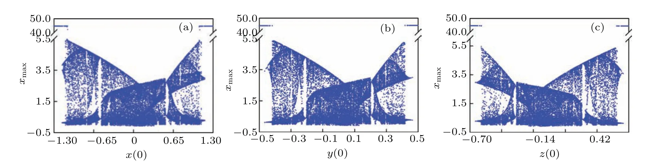
Fig. 7. Bifurcation diagrams with (a) (x(0), 0, 0, 0, 0), x(0)∈(−1.3,1.3), (b) (0, y(0), 0, 0, 0), y(0)∈(−0.5,0.5); and (c) (0, 0,z(0), 0, 0),z(0)∈(−0.7,0.7),respectively.

Assume that the system parameters are from expression(3),then the bifurcation diagrams of the conventional initial values will be calculated and depicted in Fig. 7, where we can see that although the initial terms and the ranges of its variation are different,the system motion types look similar,i.e., the motion evolves from the LP into the chaos, then back to the LP. The structure of chaotic band in Fig. 7(a) is almost the same as that in Fig. 7(b), and the chaotic band in Fig.7(c)is like a mirror image of the structure of chaotic band in Fig. 7(a) or Fig. 7(b). The difference in the chaotic zone will cause chaotic attractors of different topological structures.Considering that three conventional initial values represent the voltage or current values of different components,it is believed that the difference in the structure of the chaotic zone is caused by the nature of each dynamic element. In addition, the corresponding Lyapunov exponents are also calculated and illustrated,where the curves are similar to those in Fig.8,since the Lyapunov exponents of the LP and chaos are (0,−,−,−,−)and(+,0,−,−,−),respectively.

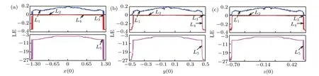
Fig. 8. Lyapunov exponent spectra with: (a) (x(0), 0, 0, 0, 0), x(0)∈(−1.3,1.3); (b) (0, y(0), 0, 0, 0), y(0)∈(−0.5,0.5); and (c) (0, 0,z(0), 0, 0),z(0)∈(−0.7,0.7),respectively.

4.2. Multistability via voltage–current model

In this subsection, the multistable characteristics of the system are revealed through the basin of attraction corresponding to the voltammetry model. The initial terms with different properties are selected as bivariate combinations to obtain the attraction basins as shown in Fig. 9, where dark blue, green and red color respectively represent the coexisting motions as“stable point”, “period”, and “complex motion” respectively.As the motions corresponding to the conventional initial values are similar, the motion ofxis taken for example. The periodic states include a variety of coexisting periodic states,such as coexisting left and right small period and large periodic limit cycles.

As can be seen from Fig.9,the multistable diagrams symmetric with respect to the origin are observed,which is consistent with the system symmetric characteristic and the motion states withinx(0)∈(−1.3,1.3) in Figs. 9(a), 9(b), and 9(d)are the same as in Fig.9(a). The motion in Fig.9(a)shows a“reverse S”shape,and the state distribution in Fig.9(b)shows some distortions with respect to the origin. The chaotic attractors in Figs. 9(a) and 9(b) are mainly distributed near the origin, and the motions switch quickly. On the contrary, the distribution in Fig.9(d)is in the strip-type,i.e.,the system has a stable and wide chaotic band. Distinguishingly, the stable points disappear and the color boundary is fuzzy,which means that the system is more sensitive to the memristive initial values. From Fig.9(c), the symmetry of the motion distribution about the origin disappears in the attraction basin,meanwhile,the color boundary is more blurred and a stable fixed point appears,which indicates that the system that relies on the change of the initial value of dual memristance has more complex dynamical behavior.

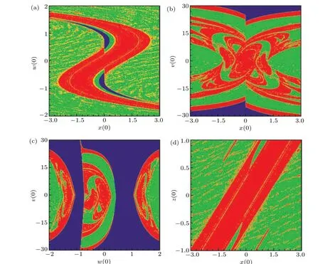
Fig.9. Attraction basins in voltage–current domain with(a)(x(0), 0, 0, w(0), 0);(b)(x(0), 0, 0, 0, v(0));(c)(0, 0, 0, w(0), v(0));and(d)(x(0), 0, z(0), 0, 0).

In summary, the dual memristive system in Eq. (2) is more sensitive to the initial value of memristive resistance.When the conventional initial value is changed,the nonlinear behavior of the system is relatively simple,and it cannot fully reflect the multistable characteristics of the system. However,the change of the initial conditions of the memristive element causes the system to produce a variety of and even an infinite number of different types of attractors, which presents better multistable characteristics.

4.3. Multistability via flux–charge model

To validate the consistency between multistabilities before and after dimensionality reduction, the attraction basin in flux–charge domain is calculated by 3OM (12) and illustrated in Figs.10,12(a),and 13(a),in which eight coexistence attractor types are observed as listed in Table 1. Figure 10 shows that the symmetry with respect to the origin still exists in Fig.10(a),but the motion distribution is distorted about the origin in Fig.10(b). The initial values of circuit elements have different effects on the motion distribution,e.g., the initial value of memristor can make the system produce more coexisting structures. With the conventional initial values varying,the chaotic behaviors are observed within a larger parameter range,but the phenomenon of multistability cannot be fully reflected. Comparing with the charge-controlled memristorM2,the motion distribution of the flux-controlled memristorM1has a wide parameter range and concentrates near the origin,so the attractor structure is more stable.

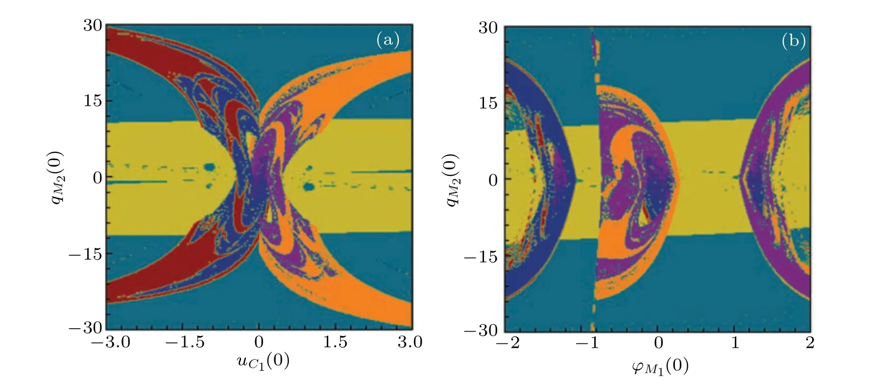
Fig.10. Two-dimensional initial value plane attraction basin for(a)uC1(0)–qM2(0)and(b)ϕM1(0)–qM2(0).

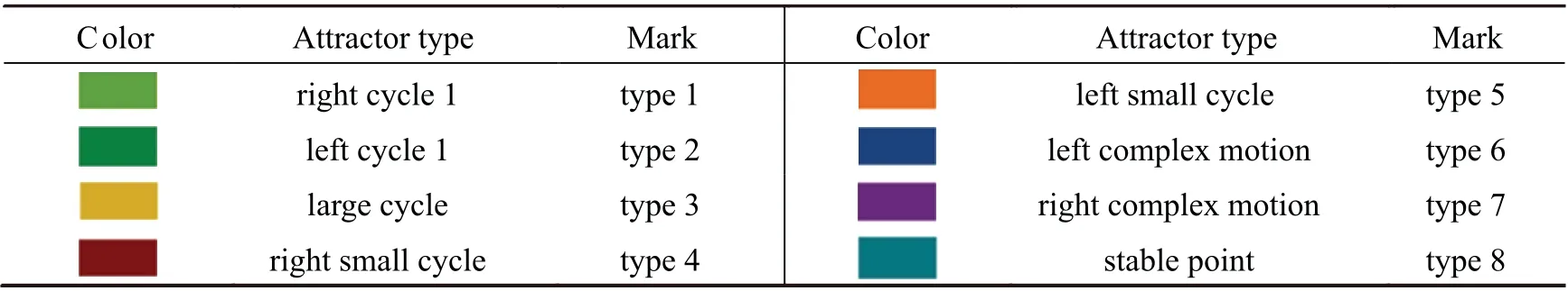
Table 1. Types of attractors in different attraction domains.

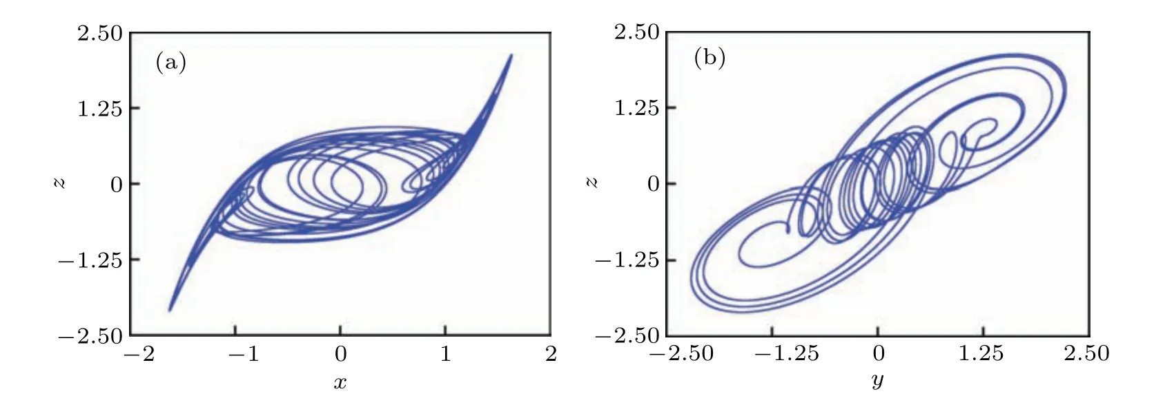
Fig.11. Chaotic attractors in planes of(a)x–z and(b)y–z.

The existence of multistability needs to be verified by the trajectory of phase plane.The chaotic attractors of 3OM under parameters in Eq.(13)are given in Fig.11 with initial conditions(0,0,0),g1=10−9,andg2=g3=0,and the coexisting attractors are also shown in Figs. 12 and 13, where different kinds of attractors can be captured by attraction basins. In Fig. 12(a), the coexistence behavior presents an ‘S’ type. In Fig.13(a),the motion distribution looks like bands and strips,which is consistent with that observed in voltage–current domain. The evolution process of the coexisting attractor corresponding to Fig. 12(a) is given in Fig. 12(b). With the increase ofuC1(0), the system trajectory changes from a large period (type 3) to a left-side cycle 1 limit cycle (type 2), and then enters into the left-side chaotic state (type 6) after multiple period bifurcation. With the increase ofuC1(0), the left chaotic attractor changes into the right chaotic attractor(type 7), then it becomes the right cycle 1 (type 1) and eventually evolves back into a large cycle limit cycle(type 3)after multiple inverse cycle bifurcations. Similarly, the coexistent attractor change process corresponding to theuC2(0)–iL(0)twodimensional initial value plane is shown in Fig.13(b). WhenuC2(0) increases from−1 to 1, the system first stabilizes in the large-cycle state(type 3), then changes into a small cycle on the left(cycle 2,type 4),and then enters into the complex motion after bicyclic cycle bifurcation has evolved into a left chaotic attractor(type 6). Subsequently,repeating the foregoing process, the attractor structure changes again into a right chaotic attractor (type 7), and then enters into a small period state (right period 2, type 5) and eventually jumps to a large period(type 3). It should be pointed out that there is a transition state of cycle 1(types 1, 2)in the movement state of the system from large cycle to small cycle.

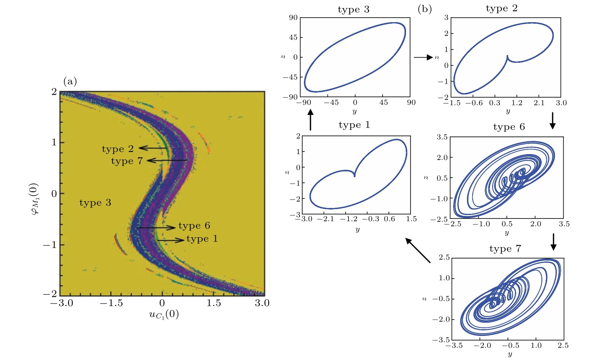
Fig.12. Evolution process of corresponding coexisting attractors in attraction basin: (a)ϕM1(0)versus uC1(0)and(b)coexisting attractors.

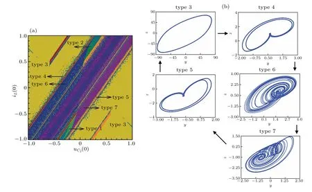
Fig.13. Evolution process of corresponding coexisting attractors in the attraction basin: (a)uC2(0)versus iL(0)and(b)coexisting attractors.

Therefore, in contrast with 5OM (in Eq. (2)), by using 3OM(in Eq.(12)),more precise and effective discussion of infinite many coexisting attractors can be obtained for the transform from initial conditions to system parameters.The motion distribution trend of the circuit on the two-dimensional initial plane before and after dimension reduction are roughly the same,in which the multistable phenomenon shows the consistency.

4.4. FPGA implementation of coexisting multistability

In this subsection, equation (12) is transformed by the FCAM, which is beneficial to the study of multistability that depends on the initial values,and its hardware memristive circuit is realized via FPGA. Analog equivalent circuit is also a way to realize the chaotic system,[27]but the setting of initial conditions is not an easy task in practice.Such a digital experiment platform can set system parameters or initial values more quickly and accurately,and is suitable for implementing memristive chaotic circuits with higher precision requirements.[28]The digital implementation of the 3OM (12) is given as follows:

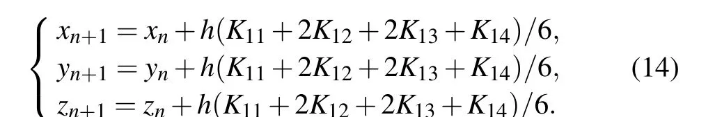
The iteration stephis set to be 0.01, andKi j(i,j=1,2,3,4)are expressed as follows:

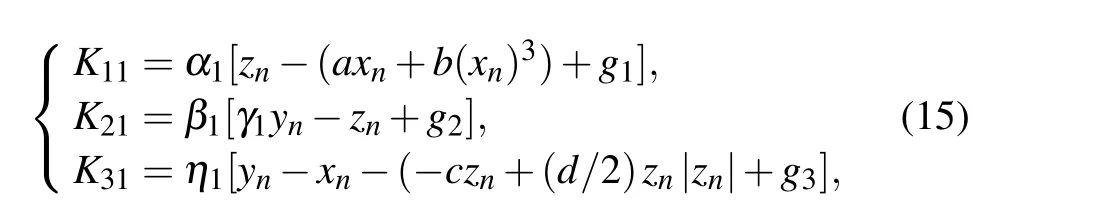
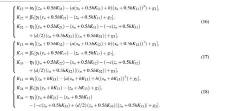
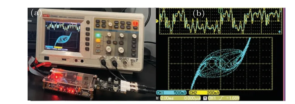
Fig. 14. FPGA implementation, showing (a) connection diagram, (b)chaotic attractor in x–z plane.

The physical connection diagram and the chaotic attractor are shown in Fig. 14. The trajectory is corresponding to that of in Fig.11(a),which verifies the correctness of numerical results. Subsequently, to reduce the multistability in the heterogeneous dual memristive circuit, a series of symmetrical coexistence attractors is presented in Fig.15,which physically realizes the unique multistability phenomenon as those shown in Figs.12 and 13. Therefore,the FPGA-based digital implementation of 3OM has high stability,good accuracy,and certain portability and universality.

Fig.15. Coexisting attractors,showing(a)left-right-period 2,(b)left-right-period 3,and(c)left-right-chaos.

5. Conclusions

In this paper, a dual-memristor-based Chua’s circuit,which shows good symmetry and multistability,is constructed by introducing two memristors with different structures. To analyze its dynamical behaviors, such as the system mechanism and the influences of the initial conditions,two analysis models,i.e.,5OM in the voltage–current domain and 3OM in the flux–charge domain, are compared with each other. The symmetric bifurcation behaviors of the DMC are first investigated in the 5OM via parameter mappings to confirm the existence of symmetry under some special system parameters.By using the 3OM, a similar symmetry with corresponding parameters is also illustrated, which partly confirms the effectiveness and correctness of FCAM in the proposed circuit.Moreover,the multistabilities in two models are observed and compared to show the coexistence of complex multiple attractors in DMC. The reliability of FCAM is validated by both numerical simulations and FPGA implementation. For engineering applications,the analysis model selection shall depend on the practical situation.