Kai Guo (郭凯), Peng-nan Sun (孙鹏楠),2, Xue-yan Cao (曹雪雁), Xiao Huang (黄潇),3

1. College of Shipbuilding Engineering, Harbin Engineering University, Harbin 150001, China,E-mail: qwertyu-147@sohu.com

2. CNR-INSEAN, Marine Technology Research Institute, Rome, Italy

3. Nuclear Engineering Program, Universidade Federal do Rio de Janeiro, Rio de Janeiro, Brazil

A 3-D SPH model for simulating water flooding of a damaged floating structure＊

Kai Guo (郭凯)1, Peng-nan Sun (孙鹏楠)1,2, Xue-yan Cao (曹雪雁)1, Xiao Huang (黄潇)1,3

1. College of Shipbuilding Engineering, Harbin Engineering University, Harbin 150001, China,E-mail: qwertyu-147@sohu.com

2. CNR-INSEAN, Marine Technology Research Institute, Rome, Italy

3. Nuclear Engineering Program, Universidade Federal do Rio de Janeiro, Rio de Janeiro, Brazil

With the quasi-static analysis method, the terminal floating state of a damaged ship is usually evaluated for the risk assessment. But this is not enough since the ship has the possibility to lose its stability during the transient flooding process.Therefore, an enhanced smoothed particle hydrodynamics (SPH) model is applied in this paper to investigate the response of a simplified cabin model under the condition of the transient water flooding. The enhanced SPH model is presented firstly including the governing equations, the diffusive terms, the boundary implementations and then an algorithm regarding the coupling motions of six degrees of freedom (6-DOF) between the structure and the fluid is described. In the numerical results, a non-damaged cabin floating under the rest condition is simulated. It is shown that a stable floating state can be reached and maintained by using the present SPH scheme. After that, three-dimensional (3-D) test cases of the damaged cabin with a hole at different locations are simulated. A series of model tests are also carried out for the validation. Fairly good agreements are achieved between the numerical results and the experimental data. Relevant conclusions are drawn with respect to the mechanism of the responses of the damaged cabin model under water flooding conditions.

Smoothed particle hydrodynamics (SPH), fluid-structure interaction, water flooding, wave-body interaction, damaged vessel

Introduction

The investigation of the transient water flooding into a damaged floating structure and the dynamic response of the latter is significant in the naval architecture and the ocean engineering[1]. This fluid-structure interacting process is closely related to the assessment of the survivability of the damaged floating structure,which loses its hull integrity under different extreme conditions, e.g. damaged by the grounding, the collision, thefreak waveimpact and the strong water jets[2-5], or attacked by underwater explosions[6-11]. In these cases, big crevasses or holes are created below the water line. The inflooding currents through these holesdecreasethe buoyancy and make thefloating structure heel and sink dynamically[12].

Usually, the sinking process of a damaged ship can be divided into three stages: the transient, progressive and steady stages[1]. During the transient stage,the water starts to rush into the structure through the damaged opening. The inflow velocity is highly dependent on the location, the scale and the shape of the damaged opening. In the second stage, i.e., the progressive stage,the flooded water continuestospread through the inner openings. This stage is dependent on theinternal geometrical characteristicsof theship.The motion of the ship is strongly coupled with the flooded water propagation. The first two stages take a short time with rapidity, accompanied with a sudden change of the forced state of the ship, which put the ship in a very dangerous situation. The third stage, i.e.,the steady state stage, comes when the flooded water,theoutside water and the structure jointly reach a steady state. Note that only when the structure is not capsized during the first two stages, the third stage can be reached. Traditionally, the quasi-static analysis method isapplied for theprediction of theterminal floating state in the steady stage. However, during the first two stages, due to the strong inflooding forces,thefloatingstructure may rolland heaveseriously,which may makethefloating structurecapsize.Therefore it is hard to predict the final floating state just by the quasi-static analysis method[13]. In addition,due to the inflooding current, considerable dynamic forces may also create secondary damages in the inner parts of the structure.

Thereweresome experimental studiesof the flooding process of a damaged ship. Manderbacka et al.[1]conducted a model test to study the flooded water and ship motions. It was shown that, at the beginning of the transient flooding process, the ship will heel dramatically towards the opposite side of the damaged opening, which heaves the hole above the water line and slows down the flooding process. Santos et al.[14]found that in an asymmetric flooding the ship might over-heel and lose its stability in the initial stage. In the study of Begovic et al.[15], an experimental assessment was made for the motions of intact and damaged ships and the model scale effect was highlighted, as an inherent problem in the experimental studies. A fullscale test was carried out by Ruponen et al.[16]to study the effect of the air compression. They found that the air in the compartment significantly delays the flooding process if the ventilations are restricted.

With the rapid development of thecomputer technology, more and more numerical methods were proposed toinvestigate the flooding processfor a damaged ship. For example, Gao et al.[17]developed a Navier-Stokes(N-S)solver combining a volume of fluid (VOF) model with the dynamic mesh technique.The freesurfaceoverturning and breaking arewell captured.However,with mesh-based methods,the dynamicmesh required for the movement of the floating body is complex in programming. Therefore,the mesh free methods are preferred.

In thelast decades,the smoothed particle hydrodynamic(SPH)method seesa rapid development and is greatly improved in accuracy, stability and efficiency[18-20]. Mainly, there are twoSPH variants,the incompressiblesmoothed particlehydrodynamic(ISPH)[21]and theweakly-compressible smoothed particlehydrodynamic(WCSPH)[22,23].Each of them hastheir own advantages.Since the internal memory is not so demanding for the WCSPH and thecodeiseasy to be paralleled,thismethod shows its potential merits in the 3-D simulations with a large quantity of particles[24].Thereweremany studiesaddressing the wave-body interactions using the SPH. In the study of Le Touzé et al.[25], the SPH wasapplied tosimulatethegreen water and ship flooding scenarios. In the study of Bouscasse et al.[26],thenonlinear water waveinteracting with floating bodies was simulated and the results were validated.Besides, the ship motions with consideration of the internalflow dynamics were recently dealt with by coupling the SPH with other CFD solvers[27,28]. In the present study, an enhanced WCSPH method is applied to investigate the dynamic behavior of a 3-D damaged floating structure. This SPH variant gives accurate and stable pressure approximations through the adoption of the diffusive terms[29-32].

In the applications for the naval architecture and the ocean engineering, with the irregular configurations of the floating structures, one comes up with the requirement of a robust boundary implementation.Thetraditionalmirroringghost boundary[23]isnot acceptable since it is hard to fill the empty area of the kernel support behind a boundary with thesimple mirroring techniques. The repulsive force boundary is a good choice, as used in Zhang et al.[13]. However the kernel truncation near the boundary might make the pressure approximation there less accurate. The normal flux boundary method proposed by De Leffe et al.[33]and applied with success in the 3-D simulation of breaking bow waves by Marrone et al.[34]is a good solution sincethekernel truncation isavoided by introducing a surface integration.Similarly,in the study of Ferrand et al.[35], an unified semi-analytical wallboundary condition wasproposed based on a renormalizing factor for writing all boundary terms. In the above two boundary treatments, only one layer of particles is needed for the boundary. It is noted that in the cases where there are particles on both sides of the wall boundary,each layer of boundary particles on each side should bedistributed,which makesthe distance between the two boundary layers larger than the radius of the kernel function, toavoid spurious interactions between the fluid particles from different sides of the wall boundary. There are also some other methodstodiscretizethewall boundary intomore than one layer of particles(with the wall thickness being at least the radius of the kernel function), such as the fixed ghost boundary in the study of Marrone et al.[36], and the coupled dynamic solid boundary treatment (SBT) algorithm in the study of Liu et al.[37]and the dummy particle boundary in the study of Adami et al.[38]. Theformer twoareconvenient for 2-D problems, and the last one is shown to be good in both 2-D and 3-D problems with freely moving boundaries,as shown by Sun et al.[39]. The one of Adami et al.[38]is finally chosen and extended for modeling the freely floating cabin wall in the present study.

Unlike the case in the study of Bouscasse et al.[26],the free movements of the floating body in the 3-D caseshave6degreesof freedom (6-DOF),which demands a robust algorithm for the coupling between the fluid and the body.In this paper,a convenient method is proposed for the evaluation of theforces applied on thefreely movingbody.Furthermore,under the actions of these hydrodynamic forces, the body movements are realized based on the translation and the rotation of the local coordinate system located on the mass center of the floating body, which allows a high accuracy for updating the position of the rigid body and strictly maintaining its shape. The present 3-Dbenchmark caseregarding thewater flooding problem can also be used for the validation of the other CFD methods in future.

1. Governing equations

In simulations of low-speed free surface flows in the field of the naval architecture and the ocean engineering, the characteristic Mach numbers are not very high, therefore, the fluid can be assumed to be barotropic, i.e., the pressure is only related to the density and the effect of the inner energy can be ignored. The governing equations are shown as follows[29]:

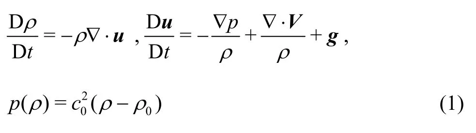
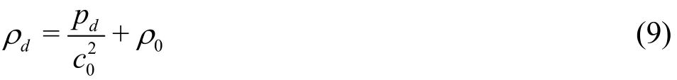
where ,u,pand refer tothedensity,the velocity,thepressureand the gravity acceleration,respectively.Vis the tensor of the viscousstress.The last equation in Eqs.(1) is an equation of state,where0ρis the reference density when the pressure of the fluid is zero on the free surface and0cis the artificial sound speed, which is a constant during the simulation.In view of both theaccuracy and the computational efficiency (sincethe timestepis restricted by the sound speed in the CFL condition),c0is defined as follows[18]

wheremaxu andmaxp arethe maximum expected velocity and pressure.

2. SPH methodology

Thefluid istreated asbarotropicand weakly compressiblein theWCSPH.Thefluid domain is discretized into a set of fluid particles. In these particles, the general variables are assigned, like the density,the pressure and the velocity.Based on these particles, the governing equations can be discretized using the kernel approximation and the particle approximation, and more theoretical details can be found in Ref.[40]. Considering the free surface effect discussed by Colagrossi et al.[41], the discretizations of the terms▽·uand p▽in Eqs.(1) are shown as follows:

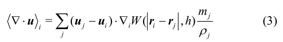
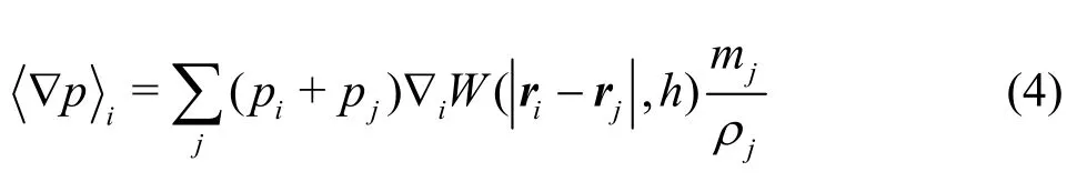
whereriis the position vector for the it h -particle and ▽iW ( ri-rj,h)isthe gradient of thekernel functionW ( ri-rj,h) with respect tothe it hparticle. The reason why we use the above two forms is that Eq.(3) keeps a good consistency near the free surfacewherethekernel function istruncated and Eq.(4) is in a good form marching Eq.(3) that keeps the energy conservation in the Hamilton system, and more details can be found in Colagrossi et al.[41]. In the present study, the Wendland C2 kernel function is adopted.The kernel function can help toavoid the occurrenceof the particle pairing instability, which was analyzed in detail in Dehnen and Aly[42]. In view of the computational efficiency, the smoothing length his set as=1.23hxΔ,wherexΔistheinitial particle spacing. To adopt more neighbors can bring a smoother velocity field and vorticity field. This was numerically investigated in Colagrossiet al.[43].Usually, in the 2-D simulations, we set =2hxΔfor the Wendland C2 kernel(50 neighboring particles),according toe.g.,Sun et al.[20].Specially,for the simulation of a standing wave in a high Reynold number,=4hxΔcan lead to a much better pressure,velocity or vorticity field[43]. But in the 3-D cases, we cannot use so large quantity of neighboring particles since the total particle number might be very large.For the cases in the present paper, we mainly focus on themotionsof the floating body.Therefore,h=1.23Δxis enough to well simulate the phenomena observed in the experiment.

The viscous force▽·Vin Eqs.(1) can be discretized into two forms in the SPH. The first form is the Morris formulation[44]shown as follows

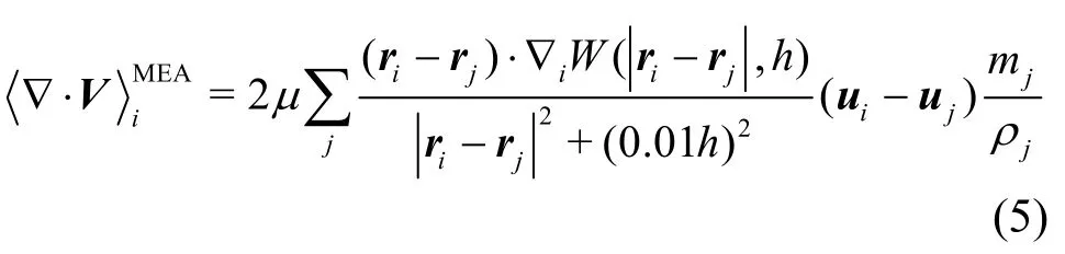
where is the dynamic viscosity. The second form is proposed by Monaghan and Gingold[45]as follows

where K = 2(d +2).According tothe analysisof Colagrossi et al.[46], Eq.(5) is not consistent near the freesurfacesince thekernel function isseriously truncated there leading toproblems with a free surface, we prefer using Eq.(6).Indeed in the present study, we only apply this term as an artificial viscosity to keep the particles distributing uniformly and to remove the velocity oscillation in order toimprove thenumerical stability and the approximation accuracy.Therefore,thedynamic viscous coefficient in Eq.(6) can be replaced byparameter.

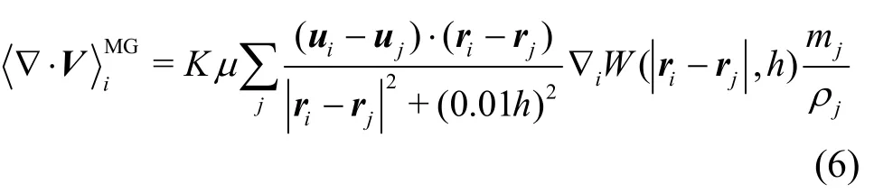
In order to avoid the spurious pressure noise, we add a diffusiveterm intothecontinuum equation.Here we apply the improved diffusive term proposed by Antuono et al.[30]. It can keep the consistency near thefree surface and avoid the rising upof the free surface particles in long-term simulations. Finally, the discretized governing equations are as follows:

where theparameters and areset tobe0.1renormalized density gradient,and more detailed explanations can be found in Randles and Libersky[47].

3. Numerical algorithms for boundary conditions

3.1 Solid wall boundary

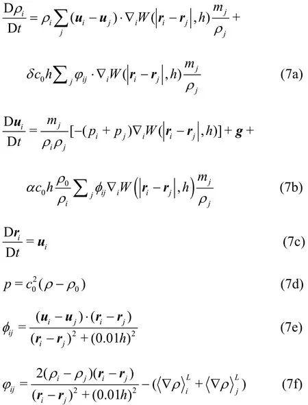
Thesolid wall boundary implementation isa traditional and difficult problem in the SPH[48,49]. In this part, we introduce the dummy particle boundary proposed by Adami et al.[38].An algorithm will be proposed in Section 3.2 to extend it to the problems with freely moving solid bodies.Thesketch of the dummy particle boundary is illustrated in Fig.1.

Fig.1 (Color online) Sketch of the dummy particle boundary for the freely moving floating body

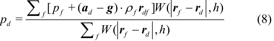
The extrapolation of thepressuredpof the dummy particle is shown as follows[38,39]

For the velocity of the dummy particle used in the approximation of the velocity divergence in the continuum equation, it is acceptable using directly the velocity of the boundarybu[38]. The velocity in the viscous term is determined based on the adoption of theboundary conditions (free-slipor no-slip).For different boundary conditions,welist thevelocity extension as follows:

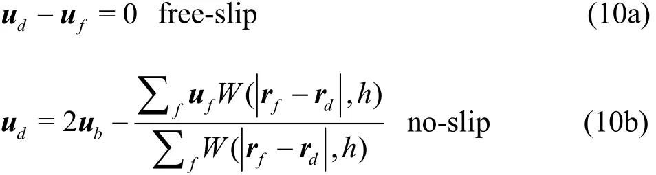
In the present study,since an artificial viscosity is applied, we adopt the free-slip boundary condition on all solid wall boundaries,including the wall of the water tank and the surface of the floating body.

3.2 Coupling interactions between the fluid and the solid body particles

Similar to the study of Bouscasse et al.[26], the approximations of the forces and the moments on the solid body are derived based on the momentum balance between thefluid and solid body particlesas follows:

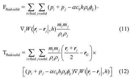
where the subscript Grefers to the gravity center of the solid body andGris the position vector of the gravity center.Thegoverningequationsfor the 6-DOF movements of the solid body are expressed as follows[50]:

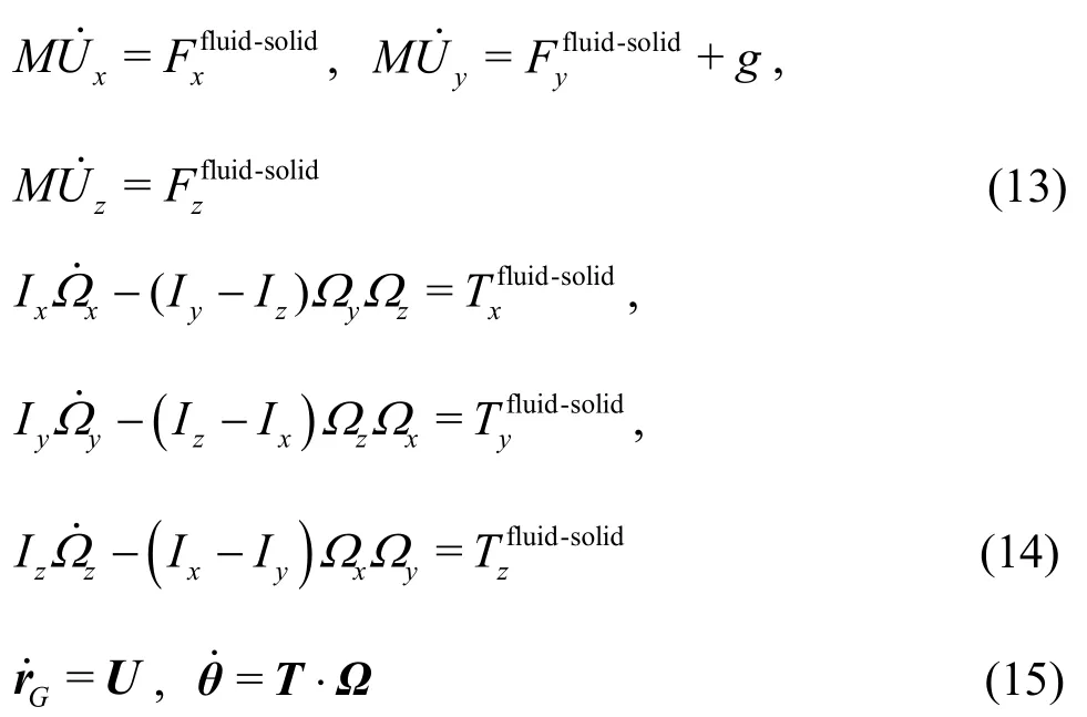
where U =(Ux, Uy, Uz)and Ω=(Ωx, Ωy, Ωz)denote the transitional and angular velocities for the solid body, respectively.θdenotes the vector of the angleof the rotation and Τisa transformation matrix which is an identity matrix in a planar motion.Mand I =(Ix, Iy, Iz)refer tothetotal massand themoment of inertia with respect tothegravity center.f˙means the time derivative of the general variable f.

We adopt a similar way as in Bouscasse et al.[26]to describe our algorithm for the fluid-body coupling.The dynamic state of the fluid particles and the body particlescan beexpressed through thevectorsfy andbyas follows:

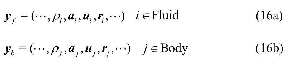
And the dynamicstateof thefloating body is expressed as

In Eqs.(16) and (17),fyandgyare updated using a 4th order Runge-Kutta integration method[30]based on Eqs.(7),(13),(14)and (15).Notethat for the second term on theleft-hand side of Eq.(14),the values predicted on the previous Runge-Kutta sub step are used. While for the components inby, as already stated in Section 3.1,jρisextrapolated from the fluid domain using Eqs.(8) and (9).juis calculated as

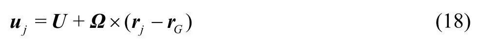
The velocity ujcalculated by Eq.(18) is used in the continuum equation.And we havetheacceleration ajfor the body particles as

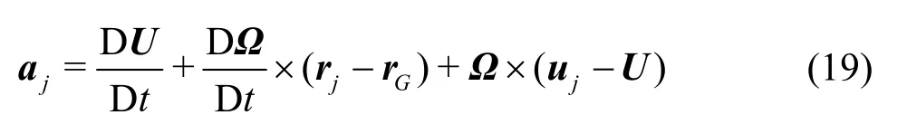
The accelerationjacalculated by Eq.(19) is used in Eq.(8)for thewall boundary implementation.In Eqs.(18)and (19),U,ΩandGr arewhat calculated at the previous Runge-Kutta sub step. Note that the updating ofjrinbyisnot based on the integration of the velocity of each body particle. In order to keep the shape of the floating body strictly unchanged, we updatejrusing first a translation of the masscenter toGrand then a rotation with the angle θat the end of each Runge-Kutta sub step.jr can be written as

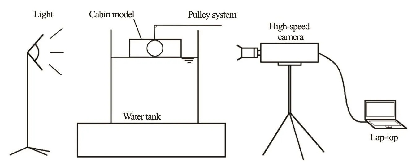
Fig.2 Sketch of the experimental setup[13]

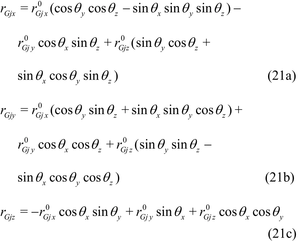
Equations (21) are obtained by an in-sequence rotatingthe position of the rigid body particle can be updated.The timestepΔtin the4thorder Runge-Kutta integration is constrained by the maximum(both the fluid and body particles) and the artificial sound speed c0

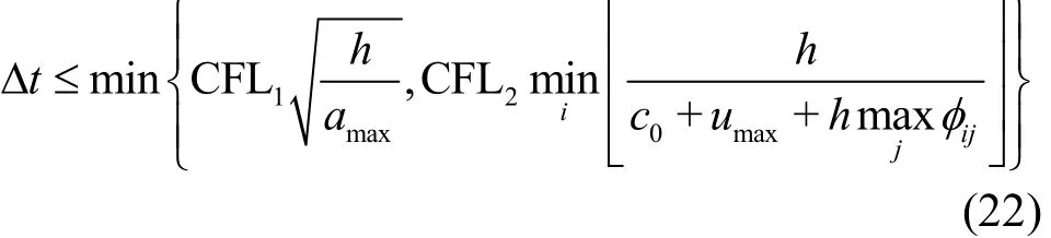
where the CFL coefficients are heuristically found as:CFL1≤0.25and CFL2≤2.0. Moreover, the parallel programming withintheOpenMP framework is basedon the study of Zhang

4. Numerical results and experimental validations

In this section, the experimental and numerical setups are presented in the first two parts. Then in the third part a test case for a non-damaged cabin model floating under the rest condition is discussed. After that, the flooding and sinking processes of one cabin model with a circular hole on its bottom and another model with the hole on its broadside are investigated,respectively.Theformer is a casewith symmetric flooding whilethe latter is onewith asymmetric flooding.Thenumerical resultsarecompared with experimental data. The pressure evolution at the probe point inside the cabin model is also measured in the SPH simulation and analyzed for a better understanding of the flooding loading process.

4.1 Experimental setup

Before the numerical simulation, a model test is carried out. The sketch of the experimental setup is shown in Fig.2. A cabin model made of PMMA with a circular holeon thebroadsideor the bottom is released by a pulley system into the water tank. As shown in the sketch, initially the bottom of the cabin model just contacts the undistributed water surface.The mass center of the cabin model is located on the vertical line that passes the center of the water tank.After releasing, the cabin model falls down and sinks dynamically under the effect of the flooding water. A high-speed camera is used to record the entire process of the water flooding and the cabin response. The data are stored in a lap-top for the post-processing with a software package. The cubic glass-made water tank has the edge length of 0.5 m, while the water depth in the tank is 0.4 m.

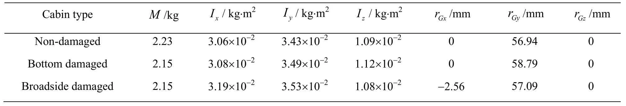
Table 1 The mass, the moment of inertia and the coordinate of mass center for

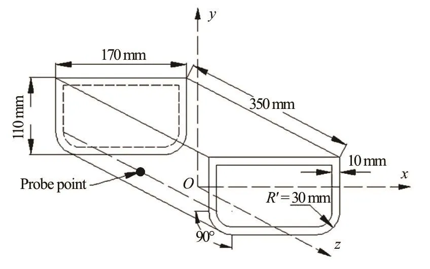
Fig.3(a) Sketch of the floating cabin model[13]

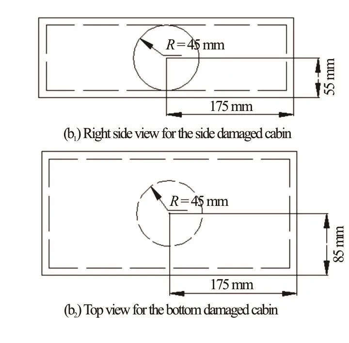
Fig.3(b) Sketch of the location of opening ho le: On the top sh ows a right side view of thebroadsidedamagedcabinand on t he bott om sh ow s the top view of th e botto m d amagedcabin.Bothoftheopeningholeshavetheradii R=45mm

Thesketch of the floating cabin model is illustrated in Fig.3. It can be seen in Fig.3(a) that each bilge of the cuboid cabin is a round chamfer with the radiusR′= 3 0mm . The cabin is 350 mm in length,170 mm in width and 110 mm in height, and the wall thickness is 10 mm. The mass, the moment of inertia and the coordinate of mass center with respect to the local coordinate axes,y,zdefined in Fig.3(a) are listed in Table 1. A probe point in the mid-ship section and on the top of the rounding bilge is also shown for measuring the pressure history in the SPH simulation.Figure3(b)showsa sketch of thelocationsof the circular opening on the broadside and on the bottom.Both the openings have the radiiR= 45mm . Moreover, on the top of the cabin models in the experiment,six small holes with the radii of 10 mm are opened for ventilation, therefore the effect of the air compression in the model test is not significant.

The non-damaged case is used to test whether the present SPH scheme can maintain a stable state for a completecabin floating under the rest condition.In the bottom damaged case, the cabin sinks dynamically with only a heaving motion. The heaving velocity is measured in the experiment and is used to validate the SPH results in Section 4.4. In the broadside damaged case,the cabin sinksdynamically with motionsin three degrees of freedom:heaving,rolling and swaying. The heaving velocity and the rolling angle are measured in the experiment and will be shown in Section 4.5 along with the SPH results.

4.2Numerical setup

In the setup of the SPH simulation, we discretize thefluid and the water tank boundary with lattice distributed particles with their regular shapes. However, the cabin model is built by the pre-processing softwarepackagein ABAQUS,sinceit is a 3-D structure with a round bilge.

Wefirst build the complete geometricmodel with the mesh, by using hexahedron elements with the edge length equal to the particle spacingxΔto be used in the SPH simulation. Afterward, we delete the nodes in the damaged hole. As an instance, the mesh for the broadside damaged cabin is shown in Fig.4(a).The node coordinates in the mesh will be read at the start of the SPH simulation, see Fig.4(b). Figure 4(c)depictsthecabin model used in theexperiment.Finally in Fig.5, the whole domain is discretized into particles with almost uniform spacing.

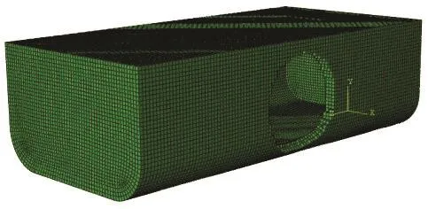
Fig.4(a) (Color online) The floating cabin model with the hole on the broadside created and meshed in ABAQUS

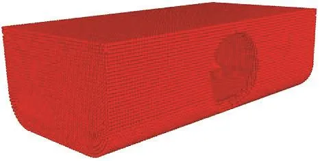
Fig.4(b) (Color online) The corresponding SPH model in the numerical simulation

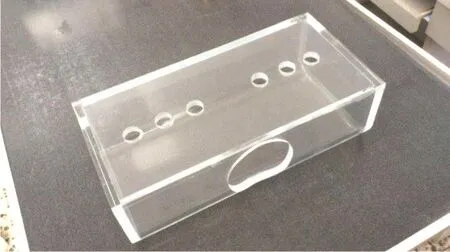
Fig.4(c) The cabin model used in the experiment[13]

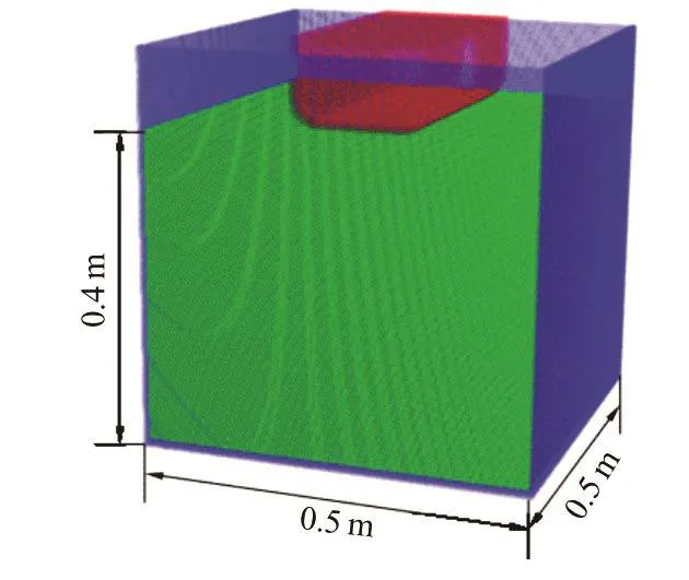
Fig.5 (Color online) The initial state in the SPH simulation

In all numerical simulations, the gravity acceleration is set asg=9.8m/s2. The density of the fluid isρ=1000kg/m3. Free-slip boundary conditions are applied on all solid wall boundaries.

4.3A non-damaged cabin floating under the rest condition

Before the hydrodynamic simulation, a numerical test case is carried out tocheck if a non-damaged cabin can maintain a stablefloating state.This test case is simple but important in demonstrating that, in fluid-solid interacting problems,themotions of the floating body are driven by the physical force instead of the numerical effect. Indeed, the SPH is good for hydrodynamicproblems,wheretheaccuracy,the stability and theconservation of theadopted SPH scheme become easy to be tested.

For a non-damaged cabin,an equilibrium state can be reached with the draughtL= 40mm. Therefore in the SPH, we start the simulation with the nondamaged modelsubmerged by 40mm.Twoparticleresolutions Δx=3.33mm and Δx=2.5mm are adopted. After a short resettlement of the particles around the model,an equilibrium state for both the cabin and the fluid is reached. In Fig.6, the floating state of the non-damaged cabin att= 2.0sis shown.The6-DOFmotionsof thecabin are measured for 2.0 s. From the time history of the velocity and the displacement in each direction shown in Fig.7 we find that the largest translational displacement isin the heaving and swaying directions (corresponding toyand coordinates). The maximum displacement is within thescale of the adopted particlespacing.Regarding the rotational motions, the rolling motionsoare most apparent. The largest rolling angles are 0.6 for Δx=3.33mm and only 0 .2ofor Δx=2.5mm.Comparing thecurvesof Δx=3.33mmand Δx=2.5mm, we find that by increasing the particle resolution, a smaller spurious motion can be observed.From the velocity curves it isshown that, with the time,theamplitudesof thevelocity oscillations decrease, as indicated in Figs.7(a) and 7(c), therefore we say that a stable floating state can be maintained within the present SPH scheme.

Fig.6 (Color online) The floating state of the non-damaged cabin at t = 2.0s (half of the domain on one side of the mid-ship section is depicted to better show the particle distribution around the cabin model)

4.4Water flooding induced responses of a bottom damaged cabin

In this part, we compare the results of the SPH simulation and the model tests for the bottom damaged case. Three different particle resolutions, Δx=3.33mm, Δx=2.5mm and Δx=2.0mm , are adopted in the SPH simulation for the convergence study.

The pressuredistribution in thefluid att=0.277sis shown in Fig.8. Although the density filter is not used, one can still find that the pressure field is stable and the spurious pressure noise is suppressed.This is due to the introduction of the artificial density diffusion in the discretized continuum equation.

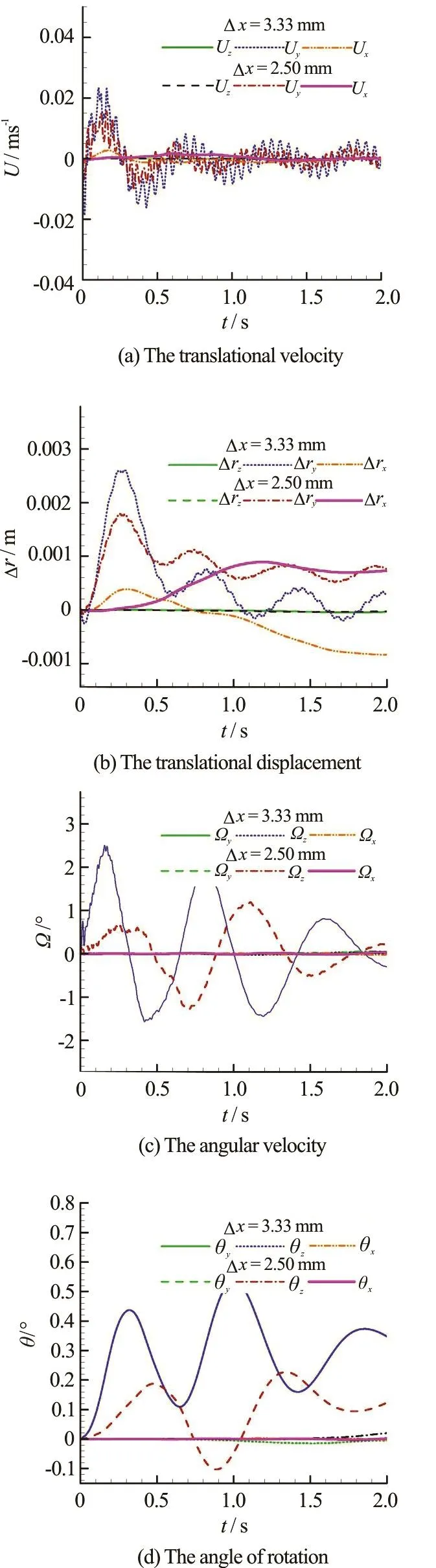
Fig.7 ( Color online) The measurements of 6-DOF motions for the non-dama-ged cabin model under the rest condition

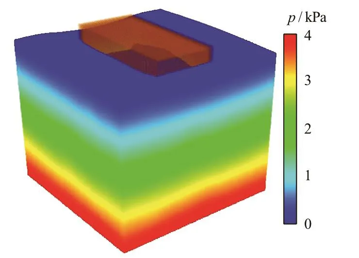
Fig.8 (Color online) The pressure contour in the fluid domain at t=0.277s

The flooding and sinking process of the bottom damaged cabin is shown in Fig.9. In the SPH results,in order to give a clearer view of the floating state and the flooding quantity, the whole fluid domain is cut at the mid-section of the floating model and only half of the domain is shown. One may find that the predicted floating state of the cabin and the flooding quantity insidethecabin agreewellwith theexperimental snapshots at different time instants. Att= 0.16s , the water starts to enter the damaged hole with the water front taking the “mushroom” shape and the 3-D SPH model well reproduces this interesting phenomenon.As the water further enters, it runs up to the broadside att= 0.24s and the water front impactson the transversebulkheadsatt= 0.34s .During the flooding process, the water wave impact and breaking areobserved and thereforethequasi-static analysis method may not be suitable for this kind of problems.Aftert= 0.79s , the inflooding water rises gradually.Att= 1.49s ,thecabin isalmost completely sunk and a similar phenomenon is also observed in the SPH snapshot.

In order togive a quantitative comparison between the numerical simulation and the model test, the timeevolution of the vertical velocityUyat the gravity center of the model is measured. As is shown in Fig.10,thecabin modelsinksgradually with a dynamically heaving motion. The SPH results agree well with the experimental data, except for the period of the oscillating velocity, which is smaller than the experimentalone,especially for therough particle resolution (Δx=3.33mm). Alsoaftert= 1.5s, the heaving velocity is a little larger than the experimental one. With the increase of the particle resolution from Δx= 3 .33mmto Δx=2.0mm ,it isfound that the discrepancy is reduced.

In the numerical calculation, the pressure history at the probe point illustrated in Fig.3(a) is measured,asshown in Fig.11.Duetotheflow impact,att= 0.2s, there is a pressure peak and after that, as the sinking process goes further on, the pressure increase is mainly due to the increase of the flooding water depth, which can also be seen fr om Fi g.9. Durin g the periodoft= 1.7s tot= 2.0s,therearesomeother pressure peaks. These pressure oscillations are originated from the hitting of the flooding water on the roof.The pressurewavereflecting inside thecabin makes the noiselast for about 0.3s.Thespurious wave reflection is an inherent problem of the WCSPH due to the adoption of a reduced speed of sound, but its negative effect on the overall movements of the floating body is negligible.

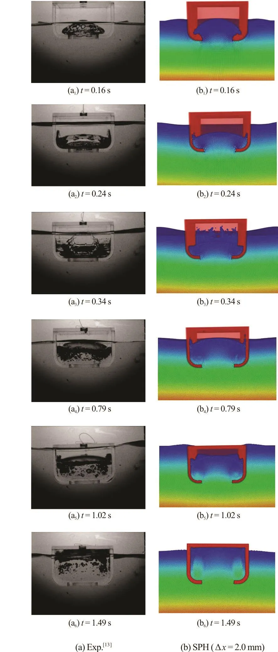
Fig.9 (Color online) The comparison at different time instants in the bottom damaged case

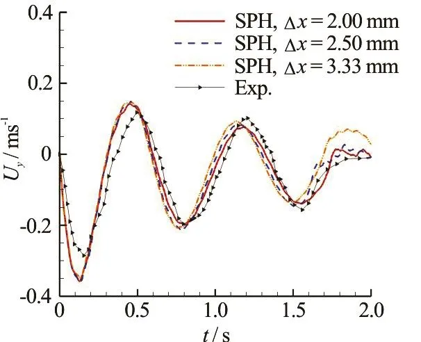
Fig.10 (Color online) Time evolution of the vertical velocity Uyin the bottom damaged case: SPH results with different particle resolutions are compared with experimental

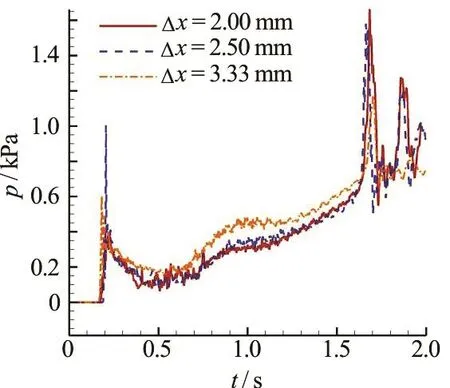
Fig.11 (Coloronline) Time evolution of the pressureon the probepointin the bottomdamaged cabin

4.5 Water flooding induced responses of a broadside damaged cabin

In this part, we make a comparison between the results of the SPH simulation and the model tests in the broadside damaged case. Three different particle resolutions,Δx =3.33mm,Δx=2.5mm ,Δx=2.0mmareadopted in theSPHsimulation.The fluid-solid interacting process is shown in Fig.12. At t = 0.25s, one can find that although more than half part of the opening hole is below the water surface,the flooding water front is rather thin compared to the“mushroom” shaped one in the bottom damaged case.Besides,thereisa water surfacehollow observed around the region near the opening hole, which is also a reason leading to the slow flooding. At t = 0.55s,theopening of thecabin model is lifted up by the buoyancy. In addition, there is a flow run-up on the left broadside of the model, which may induce a high pressureloading similar tothe mechanism of the famou sA td a tm = -b 0r.e7 a0k is n,gt h cea swea tde irs cr uu sn s-eu dp b roy l l sM daor rwonn ea nedt a process similar to the shallow water sloshing starts.The rolling angle att= 0.85s is enlarged due to the fast flooding and the inner sloshing. From the snapshots att= 1.05s andt= 2.0s, one may find that the flooding water tends to gather at the bilge on the other side of the opening, which tends to lift the damaged hole above the water surface, decrease the inflooding speed and further enlargetherolling angle.This phenomenon is consistentto the experimental findingby Manderbacka Furthermore, comparingthe position of the cabin att= 0.25s andt= 2.0sin Fig.9, a swaying motion to the right-hand side is also observed in the present study. We can deduce that the inflooding process also creates a sucking effect for the floating body,which israrely discussed in other studies. Finally, the asymmetric flooding in the broadside damaged case induces the movements of the cabin in three degrees of freedom: rolling, heaving and swaying, which is morecomplex than the previous bottom damaged one.

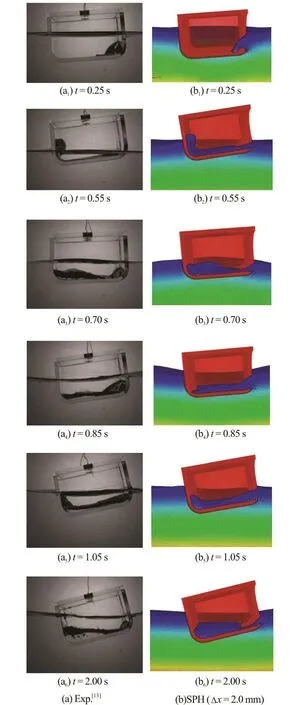
Fig.12 (Color online) The comparison at different time instants in the broadside damaged case

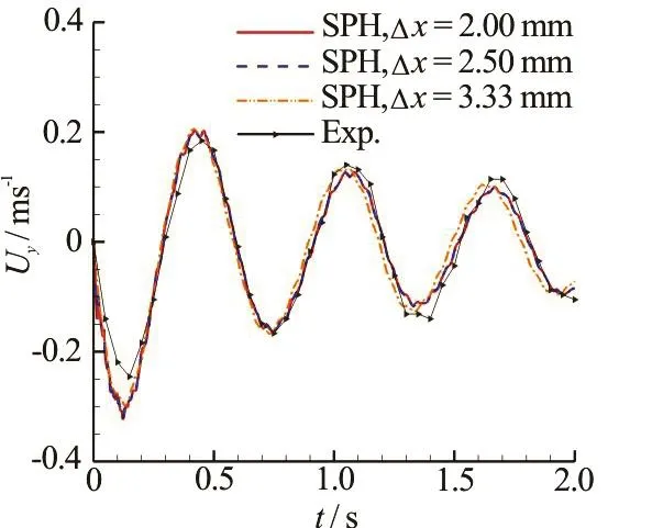
Fig.13 (Color online) Time evolution of the vertical velocity yU at the gravity center of the cabin in the broadside damaged case, SPH results are compared with the experimental results[13]

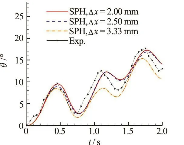
Fig.14 (Color online) Time history of the rolling angle zθ with three different particle resolutions. SPH results are compared with the experimental data[13]

The predicted time evolution of the vertical velocityUyat the gravity center of the broadside damaged cabin iscompared with experimental data in Fig.13. A fairly good agreement isachieved in the overall heaving motion of the floating body. As the particle resolution is increased, we find that the period of theoscillating velocity agreesbetter with the experimental one. Figure 14 depicts the time evolution of therolling angle.A fairly good agreement is obtained between the SPH results and the experimental data when the particle resolution Δx=2.5mmor Δx=2.0mmisadopted. The particle resolution of Δx=3.33mmis not good enough for this case. At aroundt= 1.8s, the rolling angle reaches about 1 8o,due to the flooding water gathering on one side during the inner sloshing, which is quite dangerous. Figure 15 depicts the time evolution of the swaying velocityUxand the swaying displacement Δrx. In the results of a finer particleresolution,an obviousswaying motion due to the sucking effect of the flooding water isshown,which confirmsthefindingsfrom the experimental snapshots.

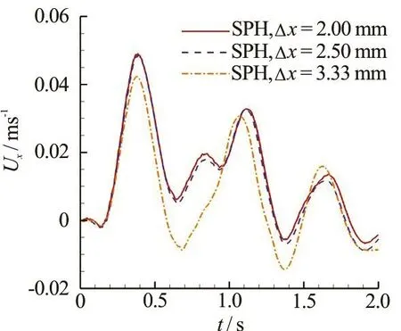
Fig.15(a) (Color online) The swaying velocity xUof the broadside damaged case

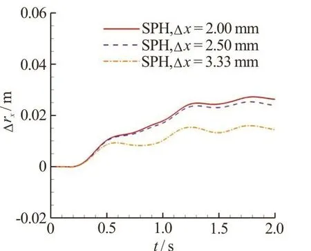
Fig.15(b) (Color online) The amplitude of the swaying motionof the broadside damaged case

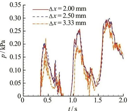
Fig.16 (Color online) Time evolutions of the pressure measured at the probe point in the broadside damaged case from the SPH simulation with three different particle resolutions

In Fig.16, the time evolution of the pressure measured at the probepoint illustrated in Fig.3(a)is shown. The pressure curve is very similar to that measured in the dam-breaking case and the shallow water sloshing case, see e.g. Marrone et al.[36]and Delorme et al.[51]. One may find that within 2 s, the pressure increases three times. It means that the inner sloshing during the sinking process is a serious issue, which deserves attention in the design of the watertight bulkhead.

5. Conclusions

In the present study, a 3-D SPH model suitable for the simulation of the water flooding into a damaged floating structure is proposed. The spurious pressure noise is avoided by applying the artificial density diffusion. The boundary implementation method is good for any irregular boundary shapes in the 3-D cases. An accurate method for evaluating the coupling motions between the floating structure and the fluid is proposed and validated. The numerical results agree well with the results of the model test, which shows the robustness of the present SPH scheme in simulating these kinds of fluid-solid interacting problems.

Firstly, a test case for the simulation of the complete cabin model floating under the rest condition is carried out, which demonstrates the capability of the present SPH scheme in maintaining the floating body in a stable state. After that, two cases of water flooding into cabins with bottom opening and broadside opening are simulated and the results are compared with the experimental data.It isfound that,in the bottom opening case, the cabin is heaving in just one degree of freedom and the cabin sinks very fast which is very dangerous and deserves attention for the ship design. In the broadside opening case,in which an asymmetric flooding process is observed, the sinking is slow because the opening hole tends to be lifted up by the rolling angle, but the dramatically rolling motion is also hazardous for the loss of stability. Besides rolling and heaving, a swaying motion is also observed in that case, which is much more complex than that in the bottom damaged case. The pressure loading inside the cabin model is measured in the SPH simulation. It is shown that in the asymmetric flooding the feature of the pressure history is very similar to the hydrodynamic loadings in the dam-breaking case and the shallow water sloshing case.

Since the model test is carried out inside a confined water tank, the boundary effect on the movements of the cabin cannot be neglected. However, the present case is a good 3-D benchmark for the test of the present SPH method in simulating water flooding problems. In the future, a transparent boundary condition which blocks the water wave reflection on the boundary can be applied in the framework of the SPH(see Shibata et al.[50]), in that case the simulation of the response of a damaged ship in a free field can be realized.Finer particleresolution along with the particle splitting and merging technique can also be applied and the flooding process of a more complex floating structure may be simulated. In addition, with the development of the multiphase SPH model, the role of the air compression in the flooding process of the damaged ship can be investigated.

Acknowledgements

This work was supported by the Ph. D. Candidate Research and Innovation Fund of theFundamental Research Funds for the Central Universities (Grant No.HEUGIP201701),thereverse-sandwich doctoral scholarship granted by FAPERJ - the State of Rio de JaneiroResearch Foundation,Brazil (Grant No.E-16/201.979/2015).

[1]Manderbacka T.,Ruponen P.,KulovesiJ.et al.Model experiments of the transient response to flooding of the box shaped barge[J]. Journal of Fluids and Structures,2015, 57: 127-143.

[2]Zhang A.M.,Liu Y.L.Improved three-dimensional bubble dynamicsmodel based on boundary element method [J]. Journal of Computational Physics, 2015, 294:208-223.

[3] Klaseboer E., Hung K., Wang C. et al. Experimental and numerical investigation of the dynamics of an underwater explosion bubble near a resilient/rigid structure [J]. Journal of Fluid Mechanics, 2005, 537: 387-413.

[4]Zhang A. M., Cui P., Cui J. et al. Experimental study on bubble dynamics subject to buoyancy [J]. Journal of Fluid Mechanics, 2015, 776: 137-160.

[5]Zhang A. M., Li S., Cui J. Study on splitting of a toroidal bubble near a rigid boundary [J]. Physics of Fluids, 2015,27(6): 062102.

[6]Zhang A. M., Zeng L. Y., Wang S. P. et al., The evaluation method of totaldamagetoshipin underwater explosion [J].Applied OceanResearch,2011,33(4):240-251.

[7]Rajendran R., Narasimhan K.Deformation and fracture behaviour of plate specimenssubjected tounderwater explosion-A review [J]. International Journal of Impact Engineering, 2006, 32(12): 1945-1963.

[8]Zhang A., Zhou W., Wang S. et al. Dynamic response of the non-contact underwater explosions on naval equipment [J]. Marine Structures, 2011, 24(4): 396-411.

[9]Zhang A.M.,Yang W.S.,Huang C.et al. Numerical simulation of column charge underwater explosion based on SPH and BEM combination [J]. Computers and fluids,2013, 71(3): 169-178.

[10] Ramajeyathilagam K., Vendhan C. Deformation and ruptureof thin rectangular platessubjected tounderwater shock [J]. International Journal of Impact Engineering,2004, 30(6): 699-719.

[11] Zhang A. M., Yang W. S., Yao X. L. Numerical simulation of underwater contact explosion [J]. Applied Ocean Research, 2012, 34: 10-20.

[12] Manderbacka T., Mikkola T., Ruponen P. et al. Transient response of a ship to an abrupt flooding accounting for the momentum flux [J].Journal of Fluids and Structures,2015, 57: 108-126.

[13] Zhang A. M., Cao X. Y., Ming F. R. et al. Investigation on a damaged ship model sinking into water based on three dimensional SPH method [J]. Applied Ocean Research,2013, 42: 24-31.

[14] Santos T., Winkle I., Soares C. G. Time domain modelling of the transient asymmetric flooding of Ro-Ro ships[J].Ocean Engineering, 2002, 29(6): 667-688.

[15] BegovicE.,Mortola G.,Incecik A.et al. Experimental assessment of intact and damaged ship motions in head,beam and quartering seas [J]. Ocean Engineering, 2013,72: 209-226.

[16] Ruponen P., Kurvinen P., Saisto I. et al. Air compression in a flooded tank of a damaged ship[J].Ocean Engineering, 2013, 57: 64-71.

[17] Gao Z., Gao Q., Vassalos D. Numerical simulation of flooding of a damaged ship[J].Ocean Engineering,2011,38(14): 1649-1662.

[18] Monaghan J. J. Smoothed particle hydrodynamics [J]. Reports on Progress in Physics, 2005, 68(8): 1703-1759.

[19] Sun P., Colagrossi A., Marrone S. et al. The δplus-SPH model: Simple procedures for a further improvement of the SPH scheme [J]. Computer Methods in Applied Mechanics and Engineering, 2017, 315: 25-49.

[20] Sun P. N., Colagrossi A., Marrone S. et al. Detection of Lagrangian coherent structures in the SPH framework [J].Computer Methods in Applied Mechanics and Engineering, 2016, 305: 849-868.

[21] Xu R., Stansby P., Laurence D. Accuracy and stability in incompressibleSPH (ISPH)based on theprojection method and a new approach [J]. Journal of Computational Physics, 2009, 228(18): 6703-6725.

[22]Zhang A.M.,Sun P. N.,Ming F.R.et al.Smoothed particle hydrodynamics and its applications in fluid-structure interactions[J].Journal of Hydrodynamics,2017.29(2): 187-216.

[23] Colagrossi A., Landrini M. Numerical simulation of interfacial flowsby smoothed particlehydrodynamics [J].Journal of Computational Physics, 2003, 191(2): 448-475.

[24] Ming F. R., Zhang A. M., Xue Y. Z. et al. Damage characteristicsof ship structuressubjected toshockwavesof underwater contact explosions[J].OceanEngineering,2016, 117: 359-382.

[25] Le Touzé D., Marsh A., Oger G. et al. SPH simulation of green water and shipflooding scenarios[J]. Journal of Hydrodynamics, 2010, 22(5): 231-236.

[26] Bouscasse B., Colagrossi A., Marrone S. et al. Nonlinear water wave interaction with floating bodies in SPH [J].Journal of Fluids and Structures, 2013, 42: 112-129.

[27]Serván-CamasB.,Cercós-Pita J.,Colom-CobbJ.et al.Time domain simulation of coupled sloshing–seakeeping problems by SPH–FEM coupling [J]. Ocean Engineering,2016, 123: 383-396.

[28] Cercos-Pita J. L., Bulian G., Pérez-Rojas L. et al. Coupled simulation of nonlinear ship motions and a free surface tank [J]. Ocean Engineering, 2016, 120: 281-288.

[29] Antuono M., Colagrossi A., Marrone S. et al. Free-surface flows solved by means of SPH schemes with numerical diffusiveterms[J].Computer Physics Communications,2010, 181(3): 532-549.

[30] Antuono M., Colagrossi A., Marrone S. Numerical diffu-sivetermsin weakly-compressibleSPH schemes[J],Computer PhysicsCommunications,2012,183(12):2570-2580.

[31] Molteni D., Colagrossi A. A simple procedure to improve the pressure evaluation in hydrodynamic context using the SPH[J].Computer Physics Communications,2009,180(6): 861-872.

[32] Cercos-Pita J., Dalrymple R., Herault A. Diffusive terms for the conservation of mass equation in SPH [J]. Applied Mathematical Modelling, 2016, 40(19): 8722-8736.

[33] De Leffe M., Le Touzé D., Alessandrini B. Normal flux method at theboundary for SPH [C].4th ERCOFTAC SPHERIC Workshop. Nantes , France, 2009.

[34] Marrone S., Bouscasse B., Colagrossi A. et al. Study of shipwave breaking patternsusing 3DparallelSPH simulations [J]. Computers and fluids, 2012, 69(4): 54-66.

[35] Ferrand M., Laurence D., Rogers B. et al. Unified semianalytical wall boundary conditions for inviscid, laminar or turbulent flows in the meshless SPH method [J]. International Journal for Numerical Methods in Fluids, 2013,71(4): 446-472.

[36] Marrone S., Antuono M., Colagrossi A. et al., δ-SPH model for simulating violent impact flows [J]. Computer MethodsinApplied Mechanics and Engineering,2011,200(13): 1526-1542.

[37] Liu M. B., Shao J. R., Chang J. Z. On the treatment of solid boundary in smoothed particlehydrodynamics[J].Science China Technological Sciences,2012,55(1):244-254.

[38] Adami S., Hu X., Adams N. A generalized wall boundary condition for smoothed particle hydrodynamics [J]. Journal of Computational Physics, 2012, 231(21): 7057-7075.

[39] Sun P., Ming F., Zhang A. Numerical simulation of interactions between free surface and rigid body using a robust SPH method [J]. Ocean Engineering, 2015, 98: 32-49.

[40] Liu M., Liu G. Smoothed particle hydrodynamics (SPH):An overview and recent developments[J]. Archives of computational Methods inEngineering,2010,17(1):25-76.

[41] Colagrossi A., Antuono M., Le Touzé D. Theoretical considerationson the free-surface rolein thesmoothedparticle-hydrodynamics model[J].Physical Review E,2009, 79(5): 056701.

[42] Dehnen W., Aly H. Improving convergence in smoothed particlehydrodynamicssimulationswithout pairing instability [J]. Monthly Notices of the Royal Astronomical Society, 2012, 425(2): 1068-1082.

[43]ColagrossiA.,Souto-IglesiasA.,AntuonoM.et al.Smoothed-particle-hydrodynamics modeling of dissipation mechanisms in gravity waves [J]. Physical Review E, 2013,87(2): 023302.

[44] Morris J. P., Fox P. J., Zhu Y. Modeling low Reynolds number incompressible flows using SPH [J]. Journal of Computational Physics, 1997, 136(1): 214-226.

[45] Monaghan J., Gingold R. Shock simulation by the particle method SPH [J]. Journal of Computational Physics, 1983,52(2): 374-389.

[46]ColagrossiA.,AntuonoM.,Souto-IglesiasA.et al.Theoretical analysis and numerical verification of the consistency of viscoussmoothed-particle-hydrodynamics formulations in simulating free-surface flows [J]. Physical Review E, 2011, 84(2): 026705.

[47] Randles P., Libersky L. Smoothed particle hydrodynamics:Some recent improvements and applications [J]. Computer Methods in Applied Mechanics and Engineering,1996,139(1-4): 375-408.

[48] Cercos-Pita J. L. AQUAgpusph, a new free 3D SPH solver accelerated with OpenCL [J].Computer Physics Communications, 2015, 192: 295-312.

[49] Liu M. B., Li S. M. On the modeling of viscous incompressible flows with smoothed particle hydro-dynamics [J].Journal of Hydrodynamics, 2016, 28(5): 731-745.

[50] Shibata K., Koshizuka S., Sakai M. et al., Lagrangian simulationsof ship-wave interactionsin rough seas[J].Ocean Engineering, 2012, 42: 13-25.

[51] Delorme L., Colagrossi A., Souto-Iglesias A. et al. A set of canonical problemsin sloshing,Part I:Pressure field inforced roll comparison between experimental results and SPH [J]. Ocean Engineering, 2009, 36: 167-178.

February 27, 2016, Revised December 9, 2016)

* Project supported by the National Natural Science Foun

dation of China (Grant Nos. U1430236, 51609045).

Biography: Kai Guo (1983-), Male, Ph. D. Candiadte,

Engineer

Peng-nan Sun,

E-mail: sunpengnan@hrbeu.edu.cn