Bin Teng (滕斌), Ying Gou (勾莹)

State Key Laboratory of Coastal and Offshore Engineering, Dalian University of Technology, Dalian 116023,China, E-mail: bteng@dlut.edu.cn

BEM for wave interaction with structures and low storage accelerated methods for large scale computation＊

Bin Teng (滕斌), Ying Gou (勾莹)

State Key Laboratory of Coastal and Offshore Engineering, Dalian University of Technology, Dalian 116023,China, E-mail: bteng@dlut.edu.cn

The boundary element method (BEM) is a main method for analyzing the interactions between the waves and the marine structures. As with the BEM, a set of linear equations are generated with a full matrix, the required calculations and storage increase rapidly with the increase of the structure scale. Thus, an accelerated method with a low storage is desirable for the wave interaction with a very large structure. A systematic review is given in this paper for the BEM for solving the problem of the wave interaction with a large scale structure. Various integral equations are derived based on different Green functions, the advantages and disadvantages of different discretization schemes of the integral equations by the constant panels, the higher order elements, and the spline functions are discussed. For the higher order element discretization method, the special concerns are given to the numerical calculations of the single-layer potential, the double layer potential and the solid angle coefficients. For a large scale computation problem such as the wave interaction with a very large structure or a large number of bodies, the BEMs with the FMM and pFFT accelerations are discussed, respectively, including the principles of the FMM and the pFFT, and their implementations in various integral equations with different Green functions. Finally, some potential applications of the acceleration methods for problems with large scale computations in the ocean and coastal engineering are introduced.

Boundary element method, Green function, accelerated BEM, wave interaction with structure

Prof. Bin Teng is now working in the State Key Laboratory of Coastal and Offshore Engineering of Dalian University of Technology. He received his Ph.D. from Dalian University of Technology in 1989, and worked as a post-doctoral research assistant in Oxford University, UK from December of 1990 to January of 1993. He received the Research Founding for Distinguished Youths in 2000, and the title of the Specially Appointed Professor in “Changjiang Scholars Programme” of Education Ministry of China in 2001. He also a Chief Scientist of a National Key Basic Research Development Program (973 Program)Project of China. He is also an associate editor of“Journal of Hydrodynamics”, and board members of“Journal of Dalian University of Technology”,“Journal of Marine Science and Application”, and“Applied Ocean Research”.

Prof. Bin Teng works on offshore and coastal hydrodynamics, including the computation of wave loads on structures, hydro-elastic analysis of very large structures, analysis of wave interaction with multiple bodies, coupling analysis of deep water platforms with risers and mooring lines, and simulation of ship berthing in harbor. He has established the second and third order wave force models in the frequency domain, and the second order and the fully nonlinear wave force models in the time-domain with higher order boundary element method.

Introduction

The interaction between waves and structures is a great concern in the coastal engineering, the ocean engineering, the naval architecture and other disciplines. The effects of the waves on the structures generally include the contribution of the water inertia,the viscosity and the free surface variation. For large-scale structures, the influence of the water viscosity is negligible, and the wave force can be solved by the potential flow theory[1]. Under the assumption of the potential flow, the wave diffraction and radiation problems can be solved with the Laplace equation and the related initial and boundary conditions. For the steady-state problem under the action of regular waves, a time factor can be separated out, and the problem can be solved in the frequency domain.

The boundary element method based on the Green's function is widely used to solve the interaction between the wave and the complex ocean engineering structures. For the frequency domain problem of the wave interaction with a structure in the horizontally unbounded domain, the integrations on the free surface, the sea bed and a vertical cylinder surface at infinity can be removed with the application of the Green function satisfying the scattering wave boundary conditions at those surfaces. Thus, with the boundary element method based on the Green function, only the body surface is required to be discretized to distribute the unknowns on the body surface. In this way, the memory requirement, the computation loads, and the tedious preparation work on meshing are greatly reduced. Therefore, the boundary element method enjoys many advantages over other domain numerical methods such as the finite element method or the finite difference method.Initially, Hess and Smith[2]introduced the constant panel method to calculate the water flow around a 3-D body, and then the method was widely used in the wave interaction with marine structures, such as:Faltinsen and Michelsen[3]and Garrison[4]et al. In the constant panel method, a 3-D body surface is discretized by a set of quadrilateral or triangular plane elements, and the unknown sources are distributed at the center of each panel and the strength of the source is constant in a panel. Finally, a set of simultaneous algebraic equations can be obtained with the application of the boundary conditions, and the strengths of the sources can thus be determined.

For a body with a curved surface, the discretized surface by a set of plane panels might not be smooth,even not continuous. In order to obtain accurate computation results, a large number of panels must be used to reduce the roughness of the body surface at the expense of the computational efficiency. In addition, the spatial derivative of the velocity potential on the body surface can not be calculated in one panel,and this will also increase the difficulty in programming and computation.

Since the late 80's of the 21th century, the higher-order boundary element methods (HOBEM)were considered to study the wave interaction with ocean structures[5-8]and ships[9,10]. In a high order boundary element method, the body surface is discretized into a set of curved quadrilateral or triangular elements. Thus, the body geometry and physical quantities, such as the velocity potential, on the body surface are expressed as functions of its nodal values by using the same shape functions. In a higher order boundary element method, the geometry of the body surface and physical quantities are continuously changing over the whole body surface.In this way, a curved body surface can be reconstructed with a small number of high order elements with high accuracy, and the same accurate potential result can be obtained with a small number of high order elements as that with a large number of constant panels. In order to balance the computational accuracy and the difficulty in the meshing preparation,the second order element is generally adopted in programming.

For the second order quadrilateral element, we can use the Lagrange interpolation method with 8 nodes or the Hermite interpolation method with 9 nodes. In the Lagrange interpolation method, the 8 nodes are generally arranged at edges and corners of a quadrilateral element, and in the Hermite interpolation method the other node is arranged at the center of the element generally. In this way, for a body discretized with NE elements, the linear algebraic equations generated by 9-nodes elements have apparently NE dimensions more than those generated by 8 nodes elements with the same number of elements. If the body geometry and the velocity potential do not change abruptly in one element, the Lagrange interpolation method will have the same accuracy as that of the Hermite interpolation method but with a higher efficiency. Therefore, the Lagrange interpolation method has more extensive applications in the hydrodynamic analysis.

Because the unknowns of a high order element method are distributed at nodes, with a continuous variation within the element, it also has the following advantages in the numerical analysis: (1) it is convenient to calculate the hydrodynamic pressure at any position on the body surface by an interpolation of the nodal values in an element and it is easy to combine a HOBEM with a finite element method for the structural analysis with different meshes, (2) the velocity potential at the waterline can be obtained directly and the wave run-up at the water-line can be computed accurately, as is required for computing the air-gap height of an offshore platform, (3) the spatial derivative of the velocity potential on the body surface can be computed easily and accurately, as is required in the calculation of the second order velocity potential and the second order force and moment on a structure.

The velocity potential and its spatial derivatives at any point in a high order element can be determined by the nodal velocity potentials with shape functions.Thus, the velocity potential is continuous on the whole body surface. The spatial derivative of the velocity potential is continuous inside the element, but not necessarily across elements. In order to make the spatial derivative of the velocity potential also consistent on the body surface, the spline functions might be used to fit the surface geometry and the velocity potential on the piecewise smooth body. One method is to use the B-spline functions to describe the coordinates of the body geometry and the velocity potential on the body surface, and to determine the expansion coefficients of the velocity potentials by the BEM. It is called the B-spline based BEM, which has been applied for the analysis for wave structure interaction problems[11,12]. The spline function is a piecewise defined polynomial function, with a high degree of smoothness at the connection points of polynomial pieces, which are called the knots, or the control points. With the application of higher order spline functions, the higher order spatial derivatives of the velocity potential can also be obtained.

When the spline functions are used in fitting a function, the local change of the function will generate variations of the simulation results in the whole domain. Because of the above characteristics, the spline function based boundary element method might be used to obtain satisfactory results with fewer pieces,but not very accurate results with the increase of the piece numbers.

In addition, for bodies with an unsmooth surface or with regions where the velocity potential changes abruptly, the body surface should be divided into several smooth patches firstly, and then the spline function is used to simulate the geometric and physical values in each patch. For a complex ocean engineering structure, how to divide the structure surface into patches is not an easy job. Therefore, the application of the spline boundary element method is not as convenient and flexible as the application of the high order boundary element method in practice.

With the development of ocean engineering, the scale of the structures becomes larger and larger, and the number of structure components is increasing greatly. There are two kinds of representative large structures, one is the very large structures to be used as the floating airports or the floating islands[13-16],such as USA's MOB and Japan's Mega Floater, the other is a group of sea wave energy conversion devices and offshore wind energy conversion turbines[17,18]. To study those problems, the BEM has a fatal weakness as its coefficient matrix is full.O(N2) operations are required to form the coefficient matrix, O (N2) computer storage to store it,and O (N2) operations to solve it, even with an iterative method, where N is the number of unknowns. For a body, if its length scale increases 10 times, its area scale will increase 100 times and the number of computation operations and the computer storage will increase 10 000 times. This growth rate will result in a large computation burden and storage requirement for computers to solve the problem of wave interaction with a large-scale structure or many bodies. For a large scale calculation, some fast algorithms with high speed and low storage were proposed, such as: the fast multipole method(FMM)[19-22], the precorrected fast Fourier transform method (pFFT)[23,24]and the wavelet transform method[25]. They can be divided into two categories in view of reducing the computer storage and speeding up calculation. One is only to store the product of the full matrix and the trial vector with an acceleration calculation method for speeding up the calculation,instead of storing the full matrix, the other is to compress the full matrix with a kind of spectral transform method, and to store a new matrix of finite bandwidth. These methods were applied to the computation of wave interaction with structures, and provide a solution to the problem of very large structures or a large number of structures. However,for different problems and calculation models,different integral equations are set up based on different Green functions. Thus, different methods and techniques have to be applied in implementing a low storage accelerated method for them.

This paper will discuss the realization skills of the FMM and pFFT methods, belonging to the first category of the low storage accelerated method, in the application for wave and structure interaction problems. The second chapter gives an introduction on the higher-order boundary element method, including the calculation skill for the singular integral in an element with the source point, and the free term in the high order element method, which is the main problem and difficulty in the implementation of a high order boundary element method, as well as in the near field analysis of the FMM and the pFFT. The third chapter introduces the accelerated methods by the Fast Multipole Method and the Precorrected Fast Fourier Transform Method for the wave interaction with structures. The section on the FMM includes the basic principle of the FMM, the implementations for the Rankine source Green function in the spherical coordinate system with the multipole decomposition and the scattering wave Green function in a finite water depth in the cylindrical coordinate system with the decomposition of Bessel functions, as well as the existing problems for the scattering wave Green function in the infinite water depth. The section on the pFFT includes the basic principle of the pFFT method,the direct implementation of the integral equations with the Rankine source Green function, and the scattering wave Green function in the infinite water depth, and the decomposition method for the implementation in the integral equation with the scattering Green function in the finite water depth. In the fourth chapter, we introduce some problems which can be solved by using the boundary element method based on the FMM and the pFFT.

1. Frequency-domain BEM for wave interaction with a body

A right-handed coordinate system Oxyz is used to study the interaction problem between waves and a body in a water depth of d. z is in the vertical upward direction and z = 0 is on the still water surface. The fluid region Ω is bounded with the free surface SF, the body surface SB, the horizontal sea bed SD, and a vertical cylindrical surface at a large distance from the body.

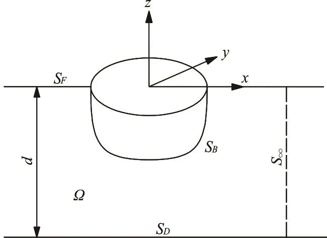
Fig.1 Sketch of definitions

It is assumed that the fluid is incompressible and the motion irrotational, so there is a potential, which satisfies the Laplace equation

For the incident waves with a regular frequency,the steady-state wave motion and the body response are all harmonic with the same frequency, under the linear approximation. Thus, the time factor can be separated out, and the velocity potential is written as

where φ(x) is the complex spatial potential function which satisfies the Laplace equation, and the following boundary conditions:

(1) The free surface condition

(2) The sea-bed condition

(3) The body surface condition

where Vnis the normal velocity at a point on the body surface.

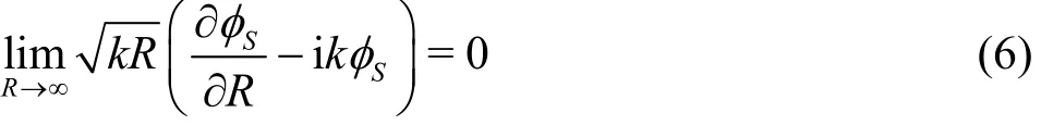
For the convenience of resolving the problem,the velocity potential is usually decomposed into the incident potential φIand the scattering potential φS.The scattering potential satisfies the Sommerfeld condition at infinity where R is the horizontal distance from the body.

With a Rankine source serving as the Green function, according to the second Green theorem, we can obtain the following integral equation

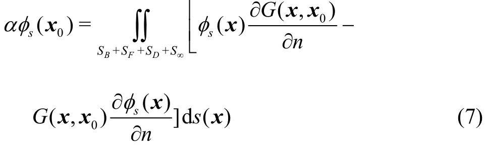
where x0and x are the coordinates of the source and the field points, and is the free term coefficient, which is also called the solid angle.

If the oscillating source satisfying the scattering wave boundary conditions is taken as the Green functio the integration on the free surface, the sea bed and the vertical cylindrical surface can be removed, and then the above integral equation is simplified as

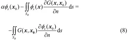
The oscillating source for the infinite water depth is

and for the finite water depth is

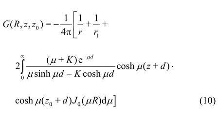
where K =ω2/g is the wave number for the infinite water depth, r is the distance between the field point and the source point, and r1is the distance between the field point and the image of the source point about the sea bed. The contour of the integration passes the singularity point from below.

The integral equation (Eq.(8)) must be resolved by a boundary element method for a structure with complex geometry. With a discretization of the body surface into NEelements, and a transformation of the discretized quadrilateral and triangular elements into standard isoparametric elements, we can write the coordinates of the body geometry and the velocity potential inside an element through its nodal values and the shape functions h (ξ,η) as:

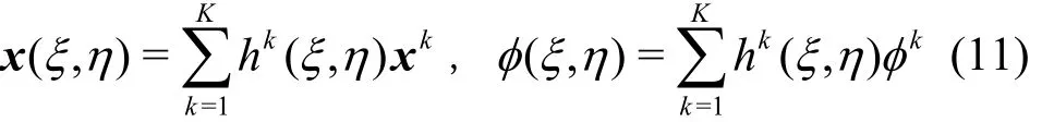
where K is the number of nodes in the element,kx andkφ are the coordinates and the potentials at nodes. In the parametric coordinate system, the integration area ds can be written as

where J (ξ,η) is the Jacobian determinant.

Substituting Eqs.(11) and (12) into the integral equation (Eq.(8)), we have

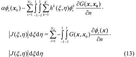
The above equation can be determined by a collocation method or the Galerkin method. With the collocation method and by arranging the source at each node over the body surface, a set of linear algebraic equations can be obtained to determine the unknown potentials at nodes over the body surface as

where N is the total number of nodes on the body surface.

For the higher order BEM equation (Eq.(13)),some special attentions must be paid to the numerical computation of the singularity integrations and the determination of the free term. The first singularity integration is the integration of the Green function in the right-hand side of Eq.(13), which is called as the single layer integration. In the element with the source point0x, the integrand will approach to infinity in the order of 1/r when the field point x approaches to the source0x. Even though the integration does exist, the direct numerical integration may involve large errors. In the numerical computation, the coordinate transform method is often used to eliminate the singular integral kernel of 1/r from the integrand.With the transformation to the polar coordinate system,the integration with a singular integral kernel of 1/r can be written as[29,30]

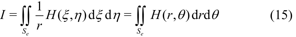
where H is a continuous finite function in the integration domain. After the coordinator transformation to remove the singularity, the integration can be dealt with by a conventional numerical integration method.

The second singular integration is the integration in the left-hand side of Eq.(13), with the derivative of the Green function, which is called as the double layer integration. When a field point x approaches to the source point x0, the derivative of the Green function approaches to infinity in the order of 1 /r2. In a constant panel method the integration of the normal derivative of the Rankine source must be zero and the integration will not make any trouble for the computation, as the panel is flat and its normal direction is perpendicular to the panel plan. While for a high order element, the integration of the normal derivative of the Green function may take a certain small value instead of zero as the element is a curved surface. In general, the integration in the element with the source point is small and can be calculated by a common numerical method.

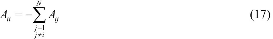
The last difficulty is the computation of the free term coefficient , or the solid angle. The physical meaning of the solid angle is the ratio of the flow discharge into the fluid domain to the total flow discharge from the source, which only depends on the local shape of the body surface at the source point. For the panel method, the source points are collocated at the centers of the flat panels, and the solid angle coefficient at any point in the center of a flat panel is equal to 1/2. But for a high order element method, the source points are collocated at the element nodes,which may be at an edge or a corner on the body surface, and the solid angle coefficient determined by the local shape of the body surface must be computed by some special techniques. The free term coefficient and the integration of the normal derivative of the Green function in the elements adjacent to the source point constitute the main diagonal terms of the matrix A, so the calculation of the main diagonal terms is difficult in applying the higher-order boundary element method.

One way of calculating the main diagonal terms is to use an indirect method, to substitute a known fiction velocity potential into the discrete integral Eq.(13), and obtain the relationship between the main diagonal terms with other off diagonal terms. For the integral equation with a closed boundary, a unit constant velocity potential can be introduced into the discretized boundary element equation, and the following relation can be obtained

Then, the main diagonal term can be computed by

For the frequency domain method for the wave interaction with a structure, the scattering wave Green function is used in the integral equation, and the integration on the free surface, the sea bed and the vertical surface at infinity are removed. The fiction potential to be used must satisfy those scattering wave conditions either. The corresponding processing methods can be found in Liu et al.[5]and Teng et al.[30,31].

For the analysis of the wave interaction with a very large structure, if a low storage accelerated method is used, the coefficient matrix A will not be set up and stored. Thus, the indirect method cannot be used, and a direct method must be adopted instead to calculate the free term coefficient. The calculation for a two-dimensional problem is relatively simple, but for a three-dimensional problem it is quite complicated. For a three-dimensional problem, the free term coefficient can be computed by the ratio of the truncated surface area of a sphere centered at the source point by the elements adjacent to the source point to the total sphere surface of24επ (Fig.2). The spherical area intercepted by the boundary elements adjacent to the source point, as shown in Fig.3, can be computed by the angleiγbetween two elements(Montic[32]) according to the theorem of the spherical geometry

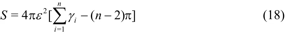
and the angleiγcan be computed by the normal directions of the two corresponding elements as

Teng et al.[30]implemented this method for the computation of the wave interaction with a 3-D structure, with the FMM and pFFT accelerated boundary element methods in the frequency-domain and time-domain analyses.

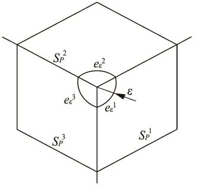
Fig.2 Elements adjacent to a source point

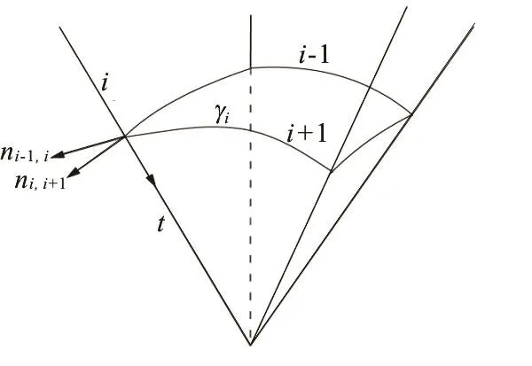
Fig.3 The angle between two elements and normal directions of the elements

2. Accelerated BEM for wave interaction with very large structures

The coefficient matrix A of the linear equations established by a boundary element method (Eq.(13))is a full matrix, which requires a storage ofO(N2),O(N2) operations for setting up it andO(N2)operations for resolving the linear equation by an iteration method, or O ( N3) operations by a direct method. A large computational burden is thus involved in solving the problem of the wave interaction with a very large structure or a large number of bodies. A fast algorithm with low storage is desirable for this problem.

The principle of the low storage acceleration method is to resolve a large set of linear equations by an iterative scheme, in which the multiplication of the matrix A and a given trial vector φkis computed by a fast calculation method, and it is stored instead of the full matrix A, thereby, the required storage is greatly reduced. For the problems of the wave interaction with structures,thefast multipole expansion method (FMM) and the pre-corrected fast transformation method (pFFT) are realized and applied.

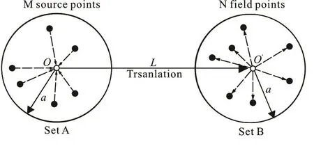
Fig.4 Definition sketch of the FMM

2.1 Fast multipole expansion accelerated BEM (FMBEM)

The FMM was proposed by Greengard and Rokhlin[19-21]for computing the interaction of a large number of point charges in the electrostatic field. It can also be used in the BEM for accelerating the computation of the source interaction companying with an iterative method to solve the linear equations.It can reduce the number of operations from O ( N2)to O(N l n N ), and the computer memory requirement from O (N2) to O (N). The essence of the FMM for computing the potentials at the field points in set B due to the sources in Set A, a distance away from Set B (Fig.4), is to expand the induced potential from one source into multiplications of the functions of the source point coordinate and those of the field point coordinate, to add the functions from all sources in Set A together, and then to determine the potential at each field point with a substitution of the coordinate of the field point. In this way, the potential at a point in Set B due to the total sources in Set A is computed all together. To compute the potential at n points in Set B due to m sources in Set A, with the FMM,O(m) + O (n ) operations are required, instead of O(m ×n) operations by the direct method. This will reduce the number of operations greatly when m and n are large.

2.2 FMBEM with Rankine source

The most simple and widely used Green function is the Rankine source. The FMM based on the Rankine source is widely applied in resolving the problems of electronics, astronomy, molecular and fluid dynamics[33-38]. The Rankine source01/(, )rxx can be expanded into multiplications of functions of the source point0x and the field point x in the spherical coordinate system about the origin O

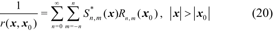
where n is the expanding order of the multipole expansion, which decides the computation accuracy and the efficiency and depends on the distance between the source point and the field point for a determined tolerance, the superscript*represents the conjugate, and the spherical harmonic functions Sn,mand Rn,mare as follows:

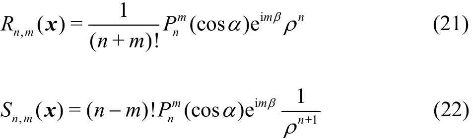
where (,,)ραβ are the spherical coordinates of the point x, i= 1- , andis the associated Legendre function.

The Rankine source is also used in the computation of the wave interaction with structures, especially in the time-domain method. Teng et al.[39,40]and Ning et al.[41]set up their FMBEM models and simulated the wave interaction with a moored floating platform in deep sea.

2.3 FMBEM with Green function in finite water depth

For the analysis of the wave interaction with a body in the frequency domain, the oscillation source which satisfies the free surface condition, the sea bed condition, and the far field condition for scattering waves is applied in the integral equation and the integration on those boundaries can be removed. Then the integration boundary is only limited to the body surface, so as to reduce the amount of calculation and storage. However, for the problem with very large structures or a large number of bodies, it is still necessary to use the fast and low storage method to accelerate the boundary element method and reduce the storage further.

In the study of the wave interaction with a very large floating body (VLFB) in the frequency domain,Utsunomiya et al.[42-44]proposed an expansion method for the wave Green function in the cylindrical coordinate system, and made a coordinate translation with the application of the Graf addition theorem. The FMM can thus be realized in the frequency domain model for the wave interaction with bodies in the finite water depth. Teng and Gou[45]implemented the method in a higher order boundary element method and used it to solve the problem of the wave interaction with multiple floating bodies.

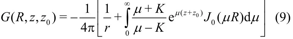
The Green's function (Eq.(10)) satisfying the scattering water conditions in a finite water depth can be written into the following series form by a transformation of the integration path[1,46]

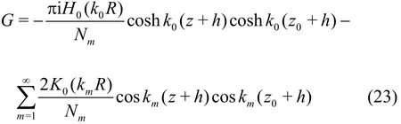
wherek0andkmare the positive and imaginary roots of the dispersive equationω2=gkt anhkh,N0=h/ 2[1+(sinh2kh/ 2kh) ],Nm≠0=h/ 2[1+(sin2km·h/ 2kmh) ],H0is the first kind of Hankel function, andK0isthe second modified Bessel function,x=(r,θ,z) andx0=(ρ,Φ,z0) are the coordinates of the field and the source points, andRis the distance between the field point and the source point.When the dimensionless distancekRis large, the convergence of the series is fast. Therefore, it can be used in the FMM for computing the effect of the sources not close to the field points.

The Green function of Eq.(23) is presented in the cylindrical coordinate system, and it is expanded with respect to the vertical eigen-functions of thezcoordinate. Next step is to expand the Hankel functionH0(k0R) and the second kind modified Bessel functionK0(kmR) in the horizontal polar coordinate system.

Take the second kind modified Bessel functionK0(kmR) as an example. In the polar coordinate system as shown in Fig.5, using the Graf's addition theorem, it takes the form as

whereIn(ρ) isthe first kind modified Bessel function ofnth order. Asφ=π +β-γ, =γα,andI-n(ρ)=In(ρ), the above equation can be written as

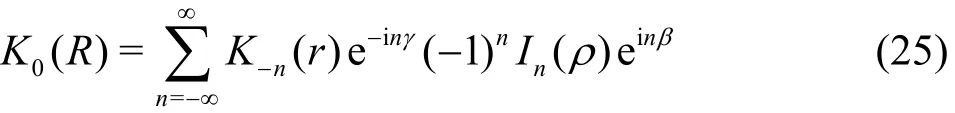
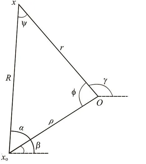
Fig.5 Definition of symbols in the coordinate translation

In applying the FMM to the free surface Green function, there are two expansion numbers which determine the efficiency, the accuracy and the storage of the acceleration method. One is the number of expansions in the Graf theorem (Eq.(24)), which assumes a small number when the field point is far from the source point, and the other is the expansion number of the eigen-functions in the vertical direction(Eq.(23)), which assumes a small number when the relative water depth (/)hLis small. With the increase of the water depth, the imaginary roots of the dispersive equation are close to each other, and become a continuous function in the infinity water.Thus, the FMM will not be efficient in the deep water and can not be implemented in this way in the infinity water.

2.4 Precorrected-FFT (pFFT) Accelerated BEM ( pFFTBEM)

The pFFT is another accelerated method[23,24].When a field point is far from the source points, the potential at the field point can be evaluated by the FFT method from the equalized sources (dipoles)distributed at the nodes of a cube grid with the same space, if the Green function satisfies a certain relationship. The number of computation operations can be reduced toO(Nl nN), whereNis the total number of the nodal knowns.

The basic process of the pFFT method is as follows, as is represented in Fig.6, where the number corresponds to a related step.

(1) Grid set-up

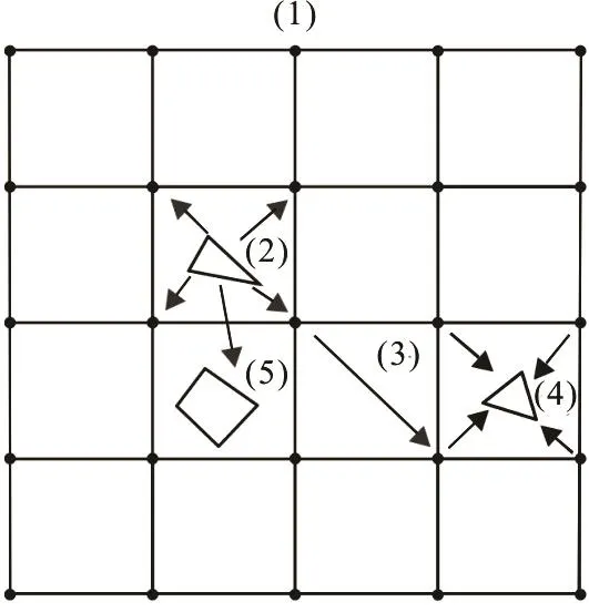
Fig.6 2-D representation of the pre-corrected-FFT method

A three-dimensional cube grid is used to surround the structure, which is divided into many small cubes with the same side length. The charges are distributed at the nodes of the grid.

(2) Projection

The sources or the dipoles at the element nodes inside a cube are projected onto the corner nodes of the cubes as the source charges. The projection standard is to generate the same potentials at some test points on a sphere surface surrounding the cube from the charges at the cube nodes and the source or dipole at the element nodes. This process is shown in Fig.7.

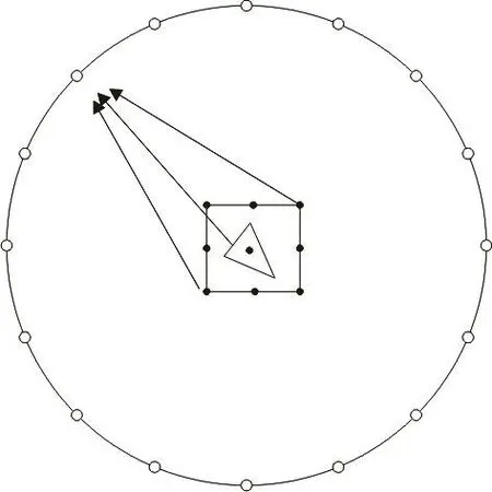
Fig.7 2-D representation of the projection scheme

(3) Calculate the grid potentials due to grid charges using FFT

Because the interval of the grid nodes is the same,the interaction of the point charges on the grid nodes can be computed by a three-dimensional discrete convolution. In this process, the Green function in the integral equation is used, and the whole calculation process is as follows

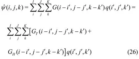
where ψˆ(i,j,k) is the velocity potential at the field point and q (i′,j′,k′) is the charge strength at the source point, I, J and K are the total numbers of grid nodes in x, y and z-directions, (i,j,k ) and(i′,j′,k′) are the indices for a field point and a source point at the grid nodes, and the difference represents the relative position of them, GTand GHare the Topelitz and Hankel matrixes formed by the Green functions. The Topelitz matrix T =[ti,j]n×nsatisfies the relation ti,j=tj,-i, and the Hankel matrix H =[hi,j]n×nsatisfies the relation hi,j=hi+1,j-1. To compute the convolution rapidly, the Green function must be represented as the functions depending only on the distance between the field and the source points.

(4) Interpolate the grid potentials onto the elements

The velocity potentials at the nodes of the boundary elements are computed by interpolation of the potentials of the grid nodes, which can also be regarded as the inverse process of the projection.

(5) Near field correction

The results obtained by interpolation of the potentials at the grid nodes also include the effect of the near field, which is not accurate and needs to be replaced. A method is to substitute the effect from the nearby cubes by the direct effect from the elements inside those cubes.

When the distance between the source point and the field point is small, the projection approximation error will be large, so the near field effect must be computed by the direct calculation method. As the number of near field elements is not large, the amount of computation is limited.

2.5 pFFT for BEM with Rankine source

The projected charges at the nodes of the grid cube from the Rankine source satisfy the Toeplitz relation in , y and z directions, so that the BEM with the Rankine source can be implemented with the pFFT method easily. The Rankine source is usually applied in the time-domain model for the wave interaction with a body, or a domain-matched method,in which the fluid domain is divided into an inner domain close to the body where the integral equation with the Rankine source is applied and an out-domain where the eigen-function expansion, or other methods,is applied.

For the time-domain model for the wave interaction with a body, Yan and Liu[47]established a pFFT accelerated model, and studied the wave-wave interaction and the wave-body interaction in large scale. In the time-domain method, the free surface condition of the wave potential is the Dirichlet condition, and the diagonal terms of the BEM matrix corresponding to the sources on the free surface are not dominant. Thus, the convergence of the iterative method for the linear equations is not as good as that of the BEM equation with only Neumann boundary condition, as the frequency domain method. This is also true for the time-domain multipole accelerated BEM.

2.6 pFFT for BEM with the free surface green func- tion in infinite water depth

The Green function in the infinite water depth(Eq.(9)) contains two parts as the follows:

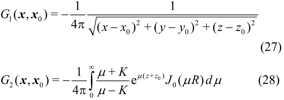
The first term is the Rankine source which can form the Toeplitz matrixes in , y and z directions and the second term of the infinite integration will form the Toepliz matrixes in and the y directions, and the Hankel matrix in z direction.Therefore, the pFFT accelerated method can be implemented in the BEM with the free surface Green function in the infinity water depth.

Korsmeyer et al.[48,49]firstly applied the pFFT method for the wave interaction with a floating body in the infinite water depth, to improve the computation efficiency and reduce the computer storage. Later, this method was used by others to study the wave interaction with very large floating structures and multi-bodies in the frequency domain, such as, Kring et al.[50], Newman and Lee[51], Dai et al.[52,53]and Jiang et al.[54].

2.7 pFFT for BEM with the free surface Green func- tion in fnite water depth

The Green function in the finite water depth(Eq.(10)) can be separated into three terms as follows:

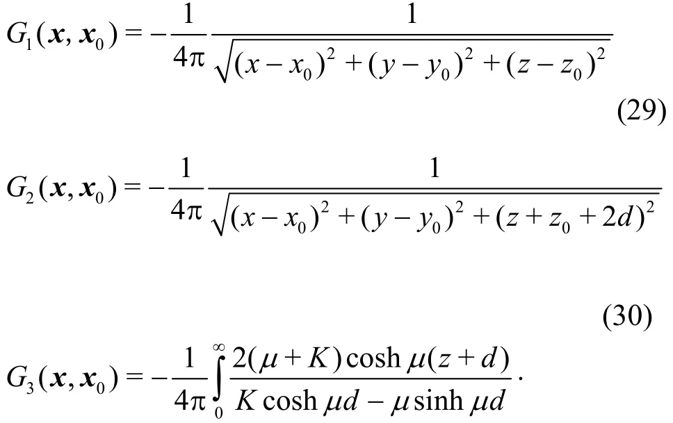
The first term is the Rankine source, from which the Toeplitz matrixes in , y and z directions can be formed. From the infinite integration of the second term, the Toepliz matrixes in and y directions,and the Hankel matrix in z direction can be formed.From the third term, the Toeplitz matrixes in and y directions can be formed, but not the Toeplitz nor the Hankel matrix in z direction. Therefore, the pFFT method can not be implemented directly for the BEM with the free surface Green function in the finite water depth.

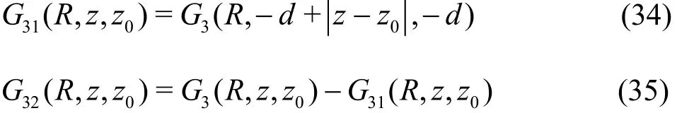
With the application of the hyperbolic function product formula, Song and Teng[55]divided the third term of the Green function into the following two parts:

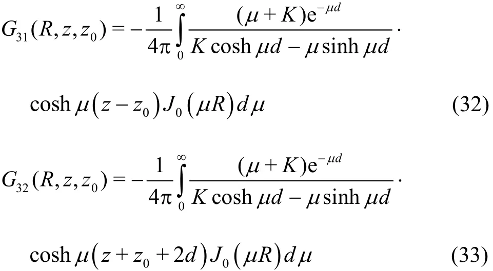
From the first part31G , the Toeplitz matrix in , y and z directions can be formed, and from the second part32G , the Toepliz matrix in and y directions,and the Hankel matrix in z direction can be formed.In this way, the boundary element method with the water surface Green function in the finite water depth can also be accelerated by the pFFT method. In the boundary element method, the Green function is computed many times, and the computation speed is the most important factor for efficiency and usefulness of a BEM. For the Green functions in the finite water depth (Eq.(10)), Newman[56]proposed a fast numerical computation method. For the new part of the Green function (Eqs.(32) and (33)), the following relations can be used in calculations by using the existing Green function code:

3. Expected applications of the lower storage and accelerated BEM

In the application of the BEM for solving the wave interaction with structures, the mesh size should be small enough to accurately describe the body geometry, the wave motion and the flow field change,especially at the corners of the body surface. Therefore, with the increase of the structure scale, the number of elements to discretize the boundary integral equation should also be increased. With the traditional boundary element method, the requirement for the storage will easily exceed the computer's capacity,and the computation time may be too long. For those kind of problems, the low storage acceleration boundary element methods might be a solution. Some examples that follow will show that the low storage accelerated BEM can be used for large computations.

3.1 Very large floating structure (VLFS)

The VLFS is a floating structure with a large horizontal scale for offshore airports or artificial islands. There are two problems in the analysis of the wave interaction with the VLFS. One is that the elastic deformation of the structure must be taken into account due to its large size and the weak stiffness of the structure, and the other is that a very large computer resource is needed to meet the requirements of the storage and the operation in the hydrodynamic analysis.

In the hydrodynamic analysis, a VLFS structure is often simplified as a two-dimensional plate with a finite length or half-infinity. Then, the eigen-function expansion method[57-60]or the Wiener Hopf method[61]is used for solving the hydrodynamic and structural response problems.

For the wave interaction with an arbitrary threedimensional large scale structure or a structure over an uneven sea bed, the above simplified analytic method will not be realizable, and a numerical method must be used. For the steady state problem of an elastic structure under the action of regular waves, the mode superposition method is widely used, in which the modal analysis of the structure is firstly carried out by a finite element method, and the elastic modes are defined as the generalized body motion modes besides the rigid body motion modes. Finally, the amplitudes of the elastic and rigid body motion modes are determined with the coupling of the rigid body motion and the elastic response equations[15,62-64]. The structure modes can be the response modes of the structure in air, called the dry modes, or the modes for the structure in water, called the wet model. It is shown that the convergent result can all be achieved for both the dry models and the wet models. Newman[65]and Eatock Taylor[66]further used the Legendre functions and the trigonometric functions to substitute the structure modes and obtained the convergent results.The foundation of this method is the hydrodynamic analysis. When the scale of a structure is large enough,a low storage and accelerated BEM must be used[43,53].

3.2 Wave interaction with a large number of bodies

Many coastal and offshore engineering structures consist of several substructures, such as a dock supported by piers and wave energy converter parks with many converters. The waves may interfere between bodies, and generate large waves around bodies, with great wave loads on bodies[67]at some special frequencies. These may threaten the safety of structures and reduce the efficiency of wave energy converters, which are arranged in groups. To solve the problem of the wave interaction with a large number of bodies is a concern and is difficult in numerical computations.

For the wave diffraction with multiply vertical cylinders, Spring and Monkneyer[68]developed an analytic solution, and Linton and Evens[69]further modified it, in which each scattering potential from a cylinder is firstly expanded into eigen-functions in the circumferential and radial directions, Fourier and Bessel functions, with respect to the origin of the coordinator system, and the expanding coefficients are determined by a set of simultaneous linear equations obtained from the body surface conditions on each cylinder.

For generalverticalaxisymmetricbodies,Kagemoto and Yue[70]used the same coupled diffraction/radiation theory,with vertical eigen expansions according to the imagery roots of the dispersion equation. Thus, a large storage of computer is required for a large number of bodies. Due to this limitation, the full coupling results were obtained only for two cylinders, and approximating solutions were obtained for 33 cylinders by taking a few Fourier expansions and neglecting the vertical expansions in their paper[70]. Göteman et al.[71]also applied the method to study the wave interaction with a large number of vertical cylindrical wave energy converters,but made further a simplification of neglecting the influence of cylinders at a certain distance, in view of computer storage and computation time.

As for an actual wave energy conversion device for extracting energy from waves, the structure is no longer a simple cylindrical structure, and some parts of the device will also move relatively with the main structure. In order to correctly simulate the working state and the energy extraction efficiency of the wave energy converters with consideration of the multiple body interference, numerical analysis methods, like the BEM, should be adopted, and be accelerated by a fast and low storage method.

3.3 Time-domain simulation

The use of the frequency domain method is only limited to steady state problems of a linear or weakly nonlinear system under the action of regular waves based on the perturbation expansion method. However,real practical problems are complex, such that the mooring system of a floating structure may have a strong nonlinearity, the wave nonlinearity may be strong, and the transient response of the structure may be a dominant factor for the safety of the structure system. For these kinds of problems, the frequency domain method is not always applicable and the time-domain model must be used instead.

Within the potential theory frame, a full-nonlinear time domain model can be set up by the BEM with the Rankine source and with the discretization on the instantaneous free surface, the instantaneous body surface and the uneven sea bed[72-74]. For further simplifying the problem and accelerating the calculation, the perturbation expansion method is also applied to set-up the first order or the second order approximation models[75,76]. As in the time-domain method, the free surface has also to be discretized with unknowns on it. Both the full-nonlinear model and the perturbation model require a large computer storage and a long computation time. It will not be practical for numerical simulations of large structures.

The FMM and the pFFT can be easily applied in the time-domain model for the simulation of the wave interaction with structures[77,78]to reduce the computer storage and accelerate the computation, as the BEM for the time domain models is based on the Rankine source. However, further study shows that the diagonal terms of the coefficient matrix of the BEM linear equations are not always dominant as the Dirichlet boundary condition is applied on the free surface. In this case the convergence of the iterative process for resolving the linear equation is slow, with a lack of computation efficiency. The remedy is to apply a high efficient iterative method for resolving the linear equation, or to derive a new integration equation with dominant diagonal terms[79].

4. Summaries

A review is given on the BEM for the wave interaction with bodies, and the accelerated methods for the BEMs with different Green functions by the FMM and the pFFT. Through the review, the following conclusions can be drawn:

(1) The integral equation can be discretized by the constant panels, the higher order elements or the spline functions. Each discretization has its advantages and disadvantages. The constant panel method is easy to be implemented, in which the singular integration of the Green function kernel can be carried out by analytical methods. However, the convergence speed of the panel method is slow, and the velocity potential is a step function from one panel to other.The spatial derivatives of the velocity potential on the body surface should be computed from the potentials of panels around the position. The high order element method enjoys a better convergence, but the computation of the singular integral of the Green function and the solid angle coefficient should be given special cares. The velocity potential changes continuously over the whole body surface, and the spatial derivative of the velocity potential can be computed inside one element, which is required for computing the high order wave force. In the spline function based BEM,the velocity potential is continuous and differentiable over the whole discrete patch. For a smooth body and a mild distribution of the velocity potential, accurate results can be obtained with a small number of pieces.However, high accurate results are hard to be achieved by increasing the number of pieces. When the structure surface is not smooth or the velocity potential changes abruptly, the structure surface should be divided into a number of patches firstly, and then the spline function is used to fit the patches.

(2) The BEMs accelerated by the FMM or the pFFT can reduce the amount of computation operations and the storage requirement from O ( N2)to O()N, where N is the total number of element nodes. For the BEM with the Rinkine source, the FMM and the pFFT can be implemented easily. For the BEM with the frequency domain Green function in the infinite depth, the pFFT can be implemented,but not the FMM. For the BEM with the frequency domain Green function in the finite depth, the FMM can be implemented in the cylindrical coordinate system, but with a slow convergence at a high frequency. The pFFT method can also be implemented,but care should be given for the decomposition of the Green function. The accelerated BEM can be applied for the wave interaction with a very large structure or a large number of bodies, like the wave energy converter park, in the frequency domain. It can be applied to the time-domain models, but the diagonal term of the BEM linear equation will not be dominant any more.

[1] Li Y. C., Teng B. Wave action on marine structures [M].Beijing, China: China Ocean Press, 2015(in Chinese).

[2] Hess J. L., Smith A. M. O. Calculation of non-lifting potential flow about arbitrary three-dimensional bodies [J].Journal of Ship Research, 1964, 8: 22-44.

[3] Faltinsen O. M., Michelsen F. C. The effect of large structures in waves at zero Froude number [C]. Proceedings Dynamics of Marine Vehicles and Structures in Waves. London, UK, 1974, 99-114.

[4] Garrison C. J. Hydrodynamic loading of large volume offshore structure: Three-dimensional source distribution method (Zienkiewicz O. C. et al. Numerical methods in offshore engineering) [M]. Chichester, UK: Wiley, 1979.

[5] Liu Y. H., Kim C. H., Kim M. H. The computation of mean drift forces and wave run-up by higher-order boundary element method [C]. The First International Offshore and Polar Engineering Conference. Edinburgh, UK, 1991,476-481.

[6] Liu Y. H., Kim C. H., Lu X. S. Comparison of higherorder boundary element and constant panel methods for hydrodynamic loadings [J]. International Journal of Offshore and Polar Engineering, 1991, 1(1): 8-17.

[7] Eatock Taylor R., Chau F. P. Wave diffraction-some developments in linear and non-linear theory [C]. Proceedings of the 10th International Conference on Offshore Mechanics and Arctic Engineering. Stavanger, Norway,1991.

[8] Teng B., Eatock Taylor R. New higher order boundary element method for wave diffraction/radiation [J]. Applied Ocean Research, 1995, 17(2): 71-77.

[9] He G. H., Chen K. M., Zhang J. S. et al. Iterative Rankine HOBEM analysis of hull-form effects in forwards-speed diffraction problem [J]. Journal of Hydrodynamics, 2017,29(2): 226-234.

[10] Xi C., Zhu R. C., Ma C. et al. Computation of linear and nonlinear ship waves by higher-order boundary element method [J]. Ocean Engineering, 2016, 114: 142-153.

[11] Maniar H. D. A three dimensional higher order panel method based on B-splines[D].Doctoral Thesis,Cambirdge, MA, USA: Massachusetts Institute of Technology, 1995.

[12] Teng B., Bai W. A B-spline based BEM and its application in predicting wave forces on 3D bodies [J]. China Ocean Engineering, 1999, 13(3): 257-264.

[13] Newman J. N., Maniar H. D., Lee C. H. Analysis of wave effects for very large floating structures [C]. The International Workshop on Very Large Floating Structures(VLFS'96). Hayama, Japan, 1996, 135-142.

[14] Ohkusu M., Nanba Y. Analysis of hydroelastic behavior of a large floating platform of thin plate configuration in waves [C]. The International Workshop on Very Large Floating Structures (VLFS'96). Hayama, Japan, 1996,143-148.

[15] Liu Y. Z., Cui W. C., Wu Y. S. Hydroelasticity of VLFS[C]. Proceedings of the 17th National Conference on Hydrodynamics and the 6th National Congress on Hydrodynamics. Hong Kong, China, 2003, 76-89(in Chinese).

[16] Wu Y. S., Zou M. S., Tian C. et al. Theory and application of coupled fluid-structure interaction of ships in waves and ocean acoustic environment [J]. Journal of Hydrodynamics, 2016, 28(6): 923-936.

[17] Falnes J., Hals J. Heaving buoys, point absorbers and arrays [J]. Philosophical Transactions of the Royal Society,A, 2012, 370(1959): 246-277.

[18] Nihous G. C. Wave power extraction by arbitrary arrays of non-diffracting oscillating water columns [J]. Ocean Engineering, 2012, 51: 94-105.

[19] Rokhlin V. Rapid solution of integral equations of classical potential theory [J]. Journal of Computational Physics,1985, 60(2): 187-207.

[20] Greengard L., Rokhlin V. A fast algorithm for particle simulations [J]. Journal of Computational Physics, 1987,73(2): 325-348.

[21] Greengard L. The rapid evaluation of potential fields in particle systems [M]. Cambridge, MA, USA: MIT Press,1988.

[22] Korsmeyer F. T., Phillips J. R., Nabors K. et al. Some empirical results on using multipole-accelerated iterative methods to solve 3-D potential integral equations [C].Proceedings: Parallel Numerical Algorithms: Proceedings of an ICASE/LaRC Workshop. Hampton, VA, USA,1995.

[23] Nabors K., Phillips J. R. Korsmeyer F. T. et al. Multipole and Precorrected-FFT accelerated iterative methods for solving surface integral formulations of three-dimensional Laplace problems (Domain-based parallelism and problem decomposition methods in science and engineering) [M].Philadelphia, USA: Society for Industrial and Applied Mathematics, 1995.

[24] Phillips J. R., White J. K. A precorrected-FFT method for electrostatic analysis of complicated 3-D structures [J].IEEE Transactions on Computer-Aided Design, 1997,16(10): 1059-1072.

[25] Nygaard J. O., Grue J. Wavelet methods for the solution of wave-body problems [J]. Journal of Engineering Mathematics, 1998, 38(3): 323-354.

[26] John F. On the motion of floating bodies. I [J]. Communications on Pure Applied Mathematics, 1949, 2(1): 13-57.

[27] John F. On the motion of floating bodies. II [J]. Communications on Pure Applied Mathematics, 1950, 3(1): 45-101.

[28] Wehausen J. V., Laitone E. V. Surface waves [M]. Berlin,Germany: Springer-Verlag, 1960, 9: 446-778.

[29] Li H. B., Han G. M., Mang H. A. A new method for evaluating singular integrals in stress analysis of solids by the direct boundary element method [J]. International Journal of Numerical Methods in Engineering, 1985,21(11): 2071-2098.

[30] Teng B., Gou Y., Ning D. Z. A higher-order BEM for wave action with structures-direct computation of free term coefficient and CPV integral [J]. Acta Oceanologica Sinica, 2006, 28(1): 132-138.

[31] Teng B. Theory of wave interaction with structures and its application [M]. Beijing, China: China Ocean Press, 2010,549-565(in Chinese).

[32] Montic V. A new formula for the C-matrix in the Somigliana identity [J]. Journal of Elasticity, 1993, 33(3):191-201.

[33] Nabors K., WHITE J. K. Multipole-accelerated capacitance extraction algorithms for 3-D structures with multiple dielectrics [J]. IEEE Transactions Circuits and Systems I: Fundamental Theory and Applications, 1992,39(12): 946-954.

[34] Watanabe O., Hayami K. A fast solver for the boundary element method using multipole expansion [C]. Proceedings 4th BEM Technology Conference (BTEC94),JASCOME. Tokyo, Japan, 1994, 39-44(in Japanese).

[35] Nishida T., Hayami K. Application of the fast multipole method to the 3-D BEM analysis of electron guns [C].Proceedings of the 19th International Boundary Element Conference held in Rome. Rome, Italy, 1997, 613–622.

[36] Nie Z. P., Hu J., Yao H. Y. et al. The fast multipole method for vector analysis of scattering from 3-dimensional objects with complex structure [J]. Acta Electronica Sinica, 1999, 27(6): 104-109.

[37] Nishimura N., Yoshida K., Kobayashi S. A fast multipole boundary integral equation method for crack problems in 3D [J]. Engineering Analysis with Boundary Elements,1999, 23(1): 97-105.

[38] Gomez J. E., POWER H. A multipole direct and indirect BEM for 2D cavity flow at low Reynolds number [J].Engineering Analysis with Boundary Elements, 1997,19(1): 17-31.

[39] Teng B., Chen B. A multipole expansion method for current diffraction from bodies [C]. Proceeding of the Fourth International Conference on Fluid Mechanics.Dalian, China, 2004.

[40] Teng B., Ning D. Z., Gou Y. A fast multipole boundary element method for three-dimensional potential flow problems [J]. Atca Oceanologica Sinica, 2004, 23(4):747-756.

[41] Ning D. Z., Teng B., Geng B. L. Application of the accelerated desingularized BEM in water wave problems[C]. ISOPE'2005. Seoul, Korea, 2005.

[42] Utsunomiya T., Watanabe E., Nishimura N. Fast multipole algorithm for wave diffraction/radition problems and its application to VLFS in variable water depth and topography [C]. Proceedings of the 12th International Conference on Offshore Mechanics and Arctic Engineering. Rio de Janeiro, Brazil, 2001.

[43] Utsunomiya T., Watanabe E. Accelerates higher order boundary element method for wave diffraction/radiation problems and its applications [C]. The 12th International Offshore and Polar Engineering Conference. Kitakyushu,Japan, 2002, 3: 305-312

[44] Utsunomiya T, Watanabe E. Wave response analysis of hybrid-type VLFS by accelerated BEM [C]. Hydroelasticity in Marine Technology. Oxford, UK, 2003, 297-303.

[45] Teng B., Gou Y. Fast multipole expansion method and its application in bem for wave diffraction and radiation [C].The 16th International Offshore and Polar Engineering Conference. San Francisco, USA, 2006, 3: 318-325.

[46] Mei C. C., Stiassnie M., Yue D. K. P. Theory and applications of ocean surface waves, Part 1: Linear aspects [M].Singapore: World Scientific, 2005.

[47] Yan H., Liu Y. An efficient high-order boundary element method for nonlinear wave–wave and wave-body interactions [J]. Journal of Computational Physics, 2011, 230(2):402-424.

[48] Korsmeyer F. T., Phillips J. R., White J. K. Procorrected-FFT algorithm for accelerating surface wave problem [C].IWWWFB. Hamburg, Germany, 1996.

[49] Korsmeyer F. T., Klemas T., White J. K. et al. Fast hydrodynamic analysis of large offshore structures [C]. The 9th International Offshore and Polar Engineering Conference.Brest, France,1999. I: 27-34.

[50] Kring D., Korsmeyer F. T., Singer J. et al. Analyzing mobile offshore bases using accelerated boundary-element methods [J]. Marine Structures, 2000, 13(4-5): 301-313.

[51] Newman J. N., LEE C. H. Boundary-element methods in offshore structure analysis [J]. Journal of Offshore Mechanics and Arctic Engineering, 2002, 124(2): 81-89.

[52] Dai Y. Z., Song J. Z., Zeng J. et al. An Application of the precorrected-FFT method to the analysis of wave-body interaction [J]. Journal of Hydrodynamics, Ser. A, 2004,19(3): 361-369(in Chinese).

[53] Dai Y. Z., Qin C. W., Huang X. P. Hydroelastic analysis of large offshore structures based on the precorrected-FFT method [J]. Journal of Yanshan University, 2004,28(2): 150-154(in Chinese).

[54] Jiang S. C., Teng B., Gou Y. et al. Applications of precorrected-FFT method to higher-order boundary element method for wave-body problem [J]. Acta Oceanologica Sinica, 2011, 33(3): 38-46.

[55] Song Z. J., TENG B. Removing irregular frequency in the pre-corrected FFT method for wave-structues interaction[J]. Chinese Journal of Hydrodynamics, 2016, 31(4):489-495(in Chinese).

[56] Newman J. N. The approximation of free-surface Green functions [C]. The 4th International Conference on Numerical Ship Hydrodynamics. Washington DC, USA, 1985.

[57] Wu C., Watanabe E., Utsunomiya T. An eigenfunction expansion-matching method for analyzing the wave-induced responses of an elastic floating plate [J]. Applied Ocean Research, 1995, 17(5): 301-310.

[58] Sahoo T., Yip T. L., Chwang A. T. On the interaction of surface waves with a semi-infinite elastic plate [C]. The 10th International Offshore and Polar Engineering Conference. Seattle, USA, 2000, 3: 594-589.

[59] Teng B., Cheng L., Liu S. X. et al. Modified eigenfunction expression methods for interaction of water waves with a semi-infinite elastic plate [J]. Applied Ocean Research,2001, 23(6): 357-368.

[60] Xu F., Lu D. Q. An Optimization of eigenfunction expansion method for the interaction of water waves with an elastic plate [J]. Journal of Hydrodynamics, 2009, 21(4):526-530.

[61] Squire V. A., Dugan J. P., Wadhanms P. et al. Ocean waves and sea ice [J]. Annual Review of Fluid Mechanics,1995, 27: 115-168.

[62] Maeda H., Masuda K., Miyajima S. et al. Hydroelastic responses of pontoon type very large floating offshore structure [J]. Journal of the Society Naval Architects of Japan, 1995, 178: 203-212.

[63] Wu Y. S., Cui W. C. Advances in the three-dimensional hydroelasticity of ships [J]. Proceedings of the Institution of Mechanical Engineers Part M Journal of Engineering for the Maritime Environment, 2009, 223(3): 331-348.

[64] Tian C., Wu Y. S., Chen Y. Q. Numerical predictions on the hydroelastic responses of a large bulker in waves [C].The 5th International Conference on Hydroelasticity in Marine Technology. Southampton, UK, 2009, 333-346.

[65] Newman J. N. Wave effects on deformable bodies [J].Applied Ocean Research, 1994, 16(1): 47-59.

[66] Eatock Tayloy R. Wet or dry modes in linear hydroelasticity–why modes? [C]. Hydroelasticity in Marine Technology, Oxford, UK, 2003, 239-250.

[67] Maniar H. D., Newman J. N. Wave diffraction by a long array of cylinders [J]. Journal of Fluid Mechanics, 1997,339: 309-330.

[68] Spring B. H., Monkneyer P. L. Interaction of plane waves with vertical cylinders [C]. The 14th International Conference on Coastal Engineering. Copenhagen, Denmark,1974, 1828-1845.

[69] Linton C. M., Evans D. V. The interaction of waves with arrays of vertical circular cylinders [J]. Journal of Fluid Mechanics, 1990, 215: 549-569

[70] Kagemoto H., Yue D. K. P. Interactions among multiple three dimensional bodies in water waves: an exact algebraic method [J]. Journal of Fluid Mechanics, 1986, 166:189-209.

[71] Göteman M., Engström J., Eriksson M. et al. Interaction distance for scattered and radiated waves in large wave energy parks [C]. The 30th International Workshop on Water Waves and Floating Bodies. Bristol, UK, 2015.

[72] Longuet-higgins M. S., Cokelet C. D. The deformation of steep surface waves on water: I. A numerical method of computation [J]. Proceedings of the Royal Society of London, 1976, 350(1660), 1-26.

[73] Yan C., Liu Y. Z. Numerical calculation of nonlinear wave diffraction [J]. Journal of Hydrodynamics, Ser. A, 1991,6(2): 10-15(in Chinese).

[74] Bai W., Eatock Taylor R. Fully nonlinear simulation of wave interaction with fixed and floating flares structures[J]. Ocean Engineering, 2009, 36(3-4): 223-236.

[75] Isaacson M., Cheung K. F. Time-domain second-order wave diffraction in three dimension [J]. Jounal of Waterway Port Coastal and Ocean Engineering, 1992, 118(5):496-516.

[76] Bai W., Teng B. Second-order wave diffraction around 3-D bodies by a time-domain method [J]. China Ocean Engineering, 2001, 15(1): 73-85.

[77] Teng B., Ning D. Z. Application of a fast multipole BIEM for flow diffraction from a 3D body [J]. China Ocean Engineering, 2004, 18(2): 291-298.

[78] Yan H., Liu Y. An efficient high-order boundary element method for nonlinear wave–waveand wave-body interactions [J]. Journal of Computational Physics, 2011,230(2): 402-424.

[79] Teng B., Gao S. Coupling of normal and hypersingular integral equations in wave-structure interaction problems[C]. Proceeding of the 31th International Workshop on Water Waves and Floating Bodies. Plymouth, USA, 2016.

July 11, 2017, Revised July 25, 2017)

* Project supported by the National Natural Science Foundation of China (Grant Nos. 51379032, 51490672 and 51479026).

Biography: Bin Teng (1958-), Male, Ph. D., Professor