Haokun Wang ,Zuhua Xu *,Jun Zhao Aipeng Jiang ,*

1 School of Automation,Hangzhou Dianzi University,Hangzhou 310018,China

2 National Laboratory of Industrial Control Technology,Department of Control Science and Engineering,Zhejiang University,Hangzhou 310027,China

1.Introduction

Model predictive control(MPC)has been the most successful advanced control technique applied to the process industries[1,2].Similar to many other model based control algorithms,the performance of MPC is directly related to model accuracy.To achieve the desired performance,e.g.offset-free tracking,in the presence of model mismatch and/or unmeasured disturbances,a disturbance model is often required to cover the difference between the measured and the predicted output[3-10].

Integrated white noise models are usually used to describe the unmeasured disturbances to achieve offset-free control.The noise covariances are assumed to be unknown but can be obtained from the steady-state operation data[10-12].To estimate the state of the system with unmeasured disturbances,Kalman filter(KF)is widely adopted.In these approaches,system state is augmented with a disturbance term as an additional component of the state,and then applies the KF to the augmented system.Some rank conditions must be satisfied to ensure detectability of the augmented system.It is convenient to use integrated white noise models,since the modeling effort is directed to obtaining noise covariances[12].If such covariances are available,it is possible to show that there exist KF gains for different disturbance models that achieve the same closed-loop performance[12],because different augmented systems are different non-minimal realizations of the same input/output process[7].Thus,existing approaches are often adequate for handling unmeasured disturbances that enter a plant if proper statistics are available.

Though routinely adopted,the use of integrated white noise model with unknown covariances may limit closed-loop performance,especially the performance of disturbance rejection.In practical situations non-stationary disturbances are ubiquitous in the form of temporary oscillations,intermittent drifts,abrupt jumps,etc.Moreover,disturbance behavior like fluctuations of feed flow rates or feed compositions from upstream units,variations in operating conditions or product grades,changes in ambient weather conditions,etc.,are commonly witnessed patterns in process industries.In such cases,the disturbances are nonstationary in nature whose properties are time-varying,and hence it might not be possible to capture the noise dynamics just with integrated white noise models.On the other hand,sluggish transient behavior of the filter may degrade the disturbance rejection performance directly because of the bad choice of filter gains.The estimation performance of the augmented KF is related to the noise covariances.Although better estimation performance can be obtained by trial-and-error,there is no clear guideline available to choose a proper covariance in practice.One possible remedy is to calculate such covariances online from the steady-state operation data[10-12].However,steady-state operation data become unavailable if the controlled plant changes in operating conditions or loads.Even if the plant runs in the steady state,a symmetric semi-definite least-squares problem must be solved online to obtain such statistics,and this will increase the computational complexity more or less.

The purpose of this study is to propose an alternative approach to handle unmeasured disturbances that have arbitrary statistics.The motivation for this study comes from applications in the control of systems that experience strong unmeasured disturbances,however,dynamic models and/or statistics of such disturbances are difficult to obtain.In this paper,two types of optimal(in the minimum-variance unbiased(MVU)sense) filters are first introduced,and then some properties of the proposed optimal filters are analyzed.The main feature of the proposed MPC is that prior knowledge of disturbance dynamics is not required.Thus,disturbances with unknown statistics can be easily handled.As a result,part of the disturbance modeling effort can be reduced.We show that the proposed MPC can achieve offset-free control in the presence of asymptotically constant unmeasured disturbances.The introduced filters provide optimal filtering performance,and this enables the controller to better reject unmeasured disturbances.

2.Preliminaries and Motivation

2.1.Disturbance models

In practice,the following linear model is often used to describe local or global dynamics of a system:

The objective is to design an MPC based on linear model(1)to have yktrack the reference signalrin the presence of model mismatch and/or unmeasured disturbances.To achieve offset-free control,one popular approach is to augment the linear model by disturbance terms,and then design an observer to estimate both the states and the disturbances:

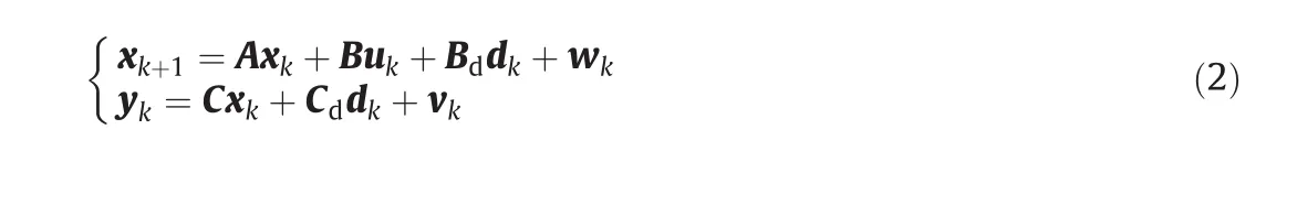
where dk∈ℝndis the disturbance term,and Bdand Cdare disturbance matrices with appropriate dimensions.Dynamics of the process noise wkcan be lumped into the disturbance term by assuming that Qk≈0.The use of model(2)provides more convenience,since both input disturbance model and output disturbance model can be represented simultaneously.A common choice of disturbance model is output disturbance model(Bd=0 and Cd=I).However,as pointed out by Shinskey[13],pure output disturbances are unlikely to occur in the process industries.In fact,the load always enters at the manipulated variable.Therefore,the following input disturbance model is often used:

Moreover,the input disturbance model(3)can represent not only input non-linearities,but also model mismatch and time-varying behaviors[7].

2.2.Linear model predictive control

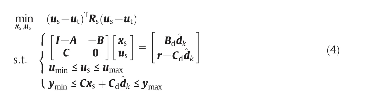
There are three main parts in the current formulations of MPC:state estimator,dynamic constrained regulator and target calculator.To guarantee a zero offset steady state,a target calculator is used to calculate the steady-state targets for the regulator[14]:

The regulation problem can be formulated by the following quadratic programming with constraints and penalties(Wx≥0and Wu≥0)[12,14]:

where uN=(uk,···,uk+N−1).The control horizon and the prediction horizon are assumed to be the same numberN,and disturbances will continue unchanged during the prediction horizon.

2.3.Kalman filter for the augmented system

In existing linear offset-free MPC schemes,the disturbance term dkis often assumed to originate from the following integrated white noise model:

Then the following steady-state KF can be used to estimate both the state and the disturbance:

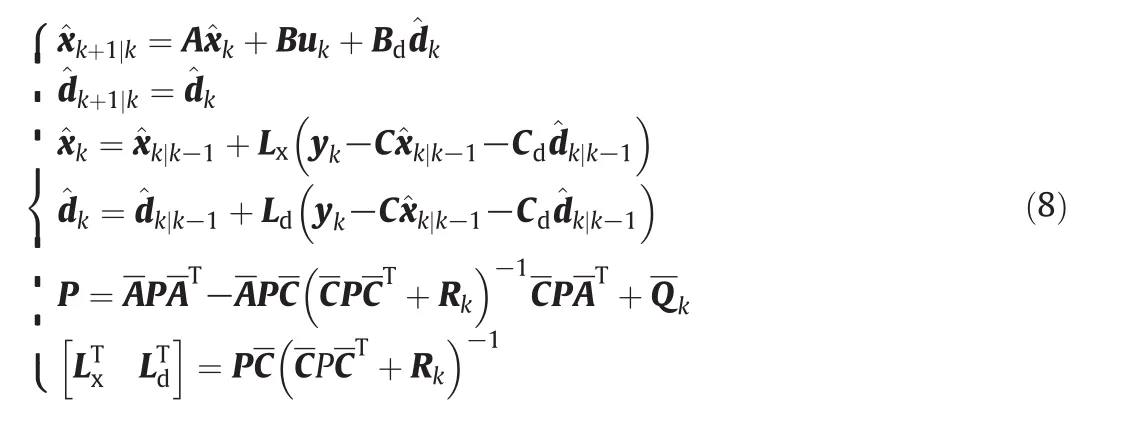
It is easy and straightforward to model disturbances using model(6),because only covariances are required.The covariances of ξk,wk,and vkare usually assumed to be unknown,however,they can be estimated from steady-state operation data[10-12].It should be noted that Skis a user-de fined parameter which is related to the estimation performance.Selecting a proper Skis of critical importance to the KFs.

2.4.Motivation

As mentioned previously,it might not be possible to capture the noise dynamics just with integrated white noise model(6)in practice.Estimation performance of the filter(Eq.(8))is usually tuned by trial-and-error,since there is no clear guideline available to choose a proper covariance.Bad choice of filter gains will degrade the estimation performance,and hence limits the control performance,especially the performance of disturbance rejection.Thus,the simple idea arises:is it possible to obtain better filtering performance if assumption(6)is relaxed?To answer the question we must identify a filter that can estimate both state and disturbances when no information(dynamic model or statistics)of disturbances is available.Fortunately,we can use linear filtering techniques[15-17]to solve the above-mentioned estimation problem.In the following section,we will focus on the design of linear optimal filters for systems with unmeasured disturbances.

3.Optimal Filter Design

By assuming that the disturbance is originated from integrated white noise model(6),output disturbance and/or input disturbance can be handled in one general framework(Eq.(8)).However,optimal filtering cannot be guaranteed with traditional KFs if dkde fies the assumed statistics.Linear MVU filtering has been proven to be a useful tool to estimate the system state and the unknown disturbance[15-17].In this section,we introduce linear MVU filters for handling dkwith arbitrary statistics.To obtain optimal filtering performance,we have to design different filters for systems(2)and(3)separately.First,optimal filter for the input disturbance model(3)is considered.Then,optimal filter for system(2)is discussed.Compared with the optimal filter for system(3),the design of optimal filter for system(2)becomes much more complicated,as the estimate error is correlated with system noise.At last,to show how the optimal filters handle disturbances with unknown statistics,the relationship between optimal filters and weighted least-squares techniques is illustrated.

Throughout this study,we assume that(A,C)is observable,(A,Q1k/2)is stabilizable,the initial state x0is of mean^x0and covariance P0,and is independent of vkfor allk.

3.1.Optimal filter for systems with input disturbance model

Considering the input disturbance model(3)with unknown disturbance statistics,the following recursive filter with control input can be used:

Including disturbance term as an additional state and assuming that disturbances are estimable,system(3)can be recast as:

The weighted least-squares solution(see[18],Chap.2.2.3)to Eq.(13)is

Substituting the gains Kkand MkofMVU filter(Eq.(9))into Eq.(14),

From Eq.(14)we can see that unmodeled dynamics and unmeasured disturbances are lumped into the augmented states x1,kin the least-squares sense.

3.2.Optimal filter for systems with input and output disturbance models

For input and output disturbance models(2),the following MVU filter for system(2)is proposed by Gillijns and De Moor[16]:

Similarly,MVU filter(Eq.(15))can be rewritten as:

Then,the weighted least-squares solution to Eq.(20)can be obtained:

Substituting Ldand Lxinto Eq.(19),one can verify that the MVU filter(Eq.(15))is equivalent to Eq.(21).

Similarly,from Eq.(21)we can see that unmodeled dynamics and unmeasured disturbances are lumped into the augmented states x2,kin the least-squares sense.This enables the MVU filters to handle disturbances with unknown statistics.Therefore,the disturbance modeling effort can be alleviated.

4.Analysis of Filter Properties

In this section,some properties of the optimal filters are analyzed.First,how many disturbances should be chosen is discussed.Second,the choice of disturbance model is addressed.Subsequently,we will demonstrate that the same estimated output can be obtained when using different disturbance models.Finally,asymptotic stability conditions are discussed.

4.1.Choice of disturbance number

From unbiasedness conditions(10)and(17),and note that Bd∈ ℝnx×ndand Cd∈ ℝny×nd,we know that the number of disturbances needs to be smaller or equal to the number of the output,that isnd≤ny.The MVU filters(Eqs.(9))and(15)can be rewritten as Eqs.(14)and(21),respectively.To ensure the existence of the optimal filters discussed in Section 3,both H1and H2must have full column rank.This also impliesnd≤ny,since(A,C)is observable.

Now we examine the choice of the disturbance in KF based approaches.The following rank condition must be satisfied to ensure the detectability of the augmented system(7)[3,4,6,7,9]:

Obviously,Eq.(22)also requires thatnd≤ny.This is equivalent to the unbiasedness conditions of optimal filters.To cover all the dynamics of the output,it is reasonable to choosend=ny.

4.2.Choice of disturbance model

After the number of disturbance is determined,we next show how to choose disturbance model pair(Bd,Cd).Usually,there is no clear guideline available to determine the disturbance model(Bd,Cd).If we use optimal filters,one is free to choose any disturbance model so long as unbiasedness conditions are satisfied.The disturbance model is often determined by experience,however,it can also be determined by solving an appropriateH∞control problem[7]or by online identification[19].

Ifnu=ny,it is easy to combine the output disturbance model and the input disturbance model,then choose as the disturbance model.In fact,disturbance model(23)is often completely adequate for handling unmeasured disturbances that enter the system.However,this does not guarantee the optimality of the disturbance model.Disturbance modeling is still an open issue.If the sources and/or dynamics of disturbances are known,a better disturbance model may be found.

4.3.Asymptotic stability analysis

We are usually concerned with asymptotic stability for the filter.In the following,asymptotic stability of the optimal filters willbe discussed.

4.3.1.Asymptotic stability of filter(Eq.(9))

Asymptotic stability of MVU filter(Eq.(9))has been discussed by Darouach and Zasadzinski[20].Sufficient conditions of asymptotic stability were also developed by Fang and de Callafon[21].Here,we give a simple result,which is equivalent to the results in[21].Now,we rewrite Eq.(11)as:

is a sufficient condition of asymptotic stability for MVU filter(Eq.(9))[21],where λi(X)is theith eigenvalue of X.

4.3.2.Asymptotic stability of filter(Eq.(15))

From Eq.(18),the estimated errors can be written as:

is a sufficient condition of asymptotic stability for MVU filter(Eq.(15)).

4.4.Global optimality analysis

It is well-known that standard KF is globally optimal,since there is no explicit constraint.This is not the case if additional constraint is imposed.In the design of MVU filters,we have shown that optimal gains are obtained by minimizing the error variance subject to unbiasedness constraints.As pointed out by Kerwin and Prince[22],the global linear minimum variance unbiased estimate may not lie within the recursive framework.Therefore,the global optimality of MVU filters needs to be reconsidered.

Now,we express the estimate of both the state and the disturbance as the most general combination of measurements and the mean of initial state:

where Fx,Fd,Γx,i,and Γd,iare combination coefficients.In existing results[15,22-24],it was proven that the optimal estimation of both the state and the disturbance for systems(3)and(2)can be written in the form of linear recursive filter as shown in Eqs.(9)and(15).Global optimality means that the proposed MVU filters are globally optimal among all possible linear filters.This enables the MPC with optimal filters to obtain better control performance,especially the performance of disturbance rejection.

5.Offset-free Tracking

In this section,we use the optimal filters discussed in Section 3 to replace KFs in existing approaches.The basic construction of the proposed MPC and existing schemes is the same and the only difference is the choice of the filter.We will show that the proposed MPC can achieve offset-free control in the presence of asymptotically constant unmeasured disturbances.

5.1.Offset-free output estimation

The above results imply that the estimated output is irrelevant to the choice of the disturbance model(Bd,Cd)if optimal filters are used.This indicates that the estimated output can track the system output in the presence of unmeasured disturbance and model mismatch.

5.2.Offset-free tracking

The offset-free tracking problem will be addressed in the proposed framework.Note that offset-free control cannot be achieved in the stochastic framework.Here we assume Qk≈0 and Rk≈0.A simple proof for offset-free control is given in the following theorem.Before the discussion,we need to make four assumptions.

Assumption 1.The target problem(4)has a unique feasible solution,and the regulation problem(5)is feasible for allk.

Assumption 2.The reference is asymptotically constant(rk→r∞),the closed-loop system reaches steady state(xk→x∞,uk→u∞,and yk→y∞).

Assumption 3.There exists a proper Bdsuch that conditions(10)and(24)for MVU filter(Eq.(9))are satisfied.

Assumption 4.There exists a proper disturbance model(Bd,Cd)such that conditions(17)and(25)for MVU filter(Eq.(15))are satisfied.

Theorem 1.If Assumptions 1–3 hold,^xk|k−1is an unbiased estimate ofxk,and the unmeasured disturbance reaches the steady-state valuedk→d∞,then the MPC(Eqs.(4)and(5))with MVU filter(Eq.(9))for system(3)can achieve the offset-free control(y∞→r∞).

Proof.Because the closed-loop system reaches steady state and the unbiasedness condition holds,unbiased estimation of xkand dkcan be obtained from the MVU filter(Eq.(9)).Therefore,we have^x∞=x∞and^d∞=d∞.The target problem(4)has a unique feasible solution which implies Cxs=r∞and xs=x∞.On the other hand,from Eq.(26)we can obtain y∞=^y∞=C^x∞.This means the predicted output^y∞is equal to the real output y∞at the steady state,i.e.y∞=^y∞=r∞.Therefore,at steady state we get the offset-free stabilization,which completes the proof.

Remark 1.By trading input non-linearities as unknown inputs,MVU filter(Eq.(9))can also be used for the control of Hammerstein systems with unknown input non-linearities[25].The proof of Theorem 1 is similar to that in Wanget al.[25].

Theorem 2.If Assumptions 1–2 and 4 hold,^xk|k−1is an unbiased estimate ofxk,and the unmeasured disturbance reaches the steady-state valuedk→d∞,thentheMPC(Eqs.(4)and(5))withMVUfilter(Eq.15)forsystem(2)can achieve the offset-free control goal(y∞→r∞).

Proof.Because the unbiasedness condition(17)holds,unbiased estimation of xkand dkcan be obtained from the MVU filter(Eq.(15)),and we can then obtain^x∞=xsand^d∞=ds.The target problem(4)has a unique feasible solution implies Cxs+Cd^d∞=r∞and xs=x∞.Then the rest of the proof is similar to Theorem 1,and is omitted for brevity.

Remark 2.When augmented KF based approaches are adopted,offsetfree control can also be guaranteed,see Muske and Badgwell[16](Theorem 4)and Maederet al.[14](Theorem 1).

The above results show that using both the input and output disturbance models(2)and input disturbance model(3)can achieve offset-free control in the proposed framework.

6.Illustrative Examples

To illustrate the performance of the proposed MPC,two examples are considered in this section.The purpose of the first one is to illustrate that even accurate disturbance model is used,the best performance cannot be guaranteed using traditional approaches.And then a distillation column model is used to show that the proposed MPC is adequate for handling model mismatch and unmeasured disturbances.

6.1.A SISO example

Here,consider an unconstrained SISO system with:A=0.3679,B=0.6321,and C=1.To demonstrate the performance of the proposed approach,we compare the proposed MPC with two KF based approaches.In KF based approaches,the system is augmented as Eq.(8),and we choose(Bd=0,Cd=I)for the output disturbance model and(Bd=B,Cd=0)for the input disturbance model.In the proposed approach,MVU filter(Eq.(15))with disturbance model(23)(Bd=B,Cd=I)is used,which can be seen as a combination of both the input and the output disturbance models.The test is under the same parameters Rk≈0,Qk≈0,Sk=I,Wx=I,Wu=I,and Rs=I.Steady-state KFs are used for both the two KF based approaches,and the corresponding filter gains are:[0;1]and[1;1.582].The set-point tracking performance of the three approaches yields no significant difference.Because disturbance rejection is much more important than set-point tracking response[13],we only consider the disturbance rejection performance in the following discussions.

6.1.1.Input step disturbance rejection

First,we add a step unmeasured disturbance to the input at time 1.We compare the above-mentioned three approaches,and the corresponding disturbance rejection performance is shown in Fig.1.From Fig.1 we can see that the approach based on the optimal filter performs better than the other two approaches.Note that an input disturbance model is an accurate description of disturbances in this case.However,as shown in Fig.1,the approach based on the input disturbance model does not provide the best performance.

Fig.1.Input disturbance rejection.

6.1.2.Output step disturbance rejection

Here,we add the same step unmeasured disturbance to the output at sampling time 1.We also consider the above three approaches,and the filter gains are the same as for the former test.The comparison of performance for output disturbance rejection is plotted in Fig.2.

Fig.2.Output disturbance rejection.

In fact,an output disturbance model is an accurate description of disturbances.However,as shown in Fig.2,the output disturbance based approach provides the worst performance.The optimal filter based approach performs better than the two KF based approaches.

It is obvious that an integrated disturbance model cannot describe step disturbances exactly,and the resulting performance is not optimal.The results presented in the above tests clearly show that best control performance cannot be guaranteed even accurate disturbance models are adopted.Better performance can be obtained if we use optimal filters to replace the KFs.

6.1.3.Stochastic disturbance rejection

We know that if dkis modeled by integrated white noise model,KF based approaches will perform very well,because KF is optimal in this case.However,such integrated white noise models are hardly warranted in practice,because the nature of the disturbances is often unknown.Now,we use a stochastic disturbance with unknown statistics as shown in Fig.3 to replace the step disturbance used in the previous tests.

Fig.3.Unmeasured stochastic disturbance.

Table 1Rejection performance under input stochastic disturbance

Performance after we added the same disturbance to the output is shown in Table 2.Similarly,we can see that the proposed approach provides the best performance.

From the above tests,we can see that the proposed MPC is adequate for rejecting both the deterministic and the stochastic disturbances that enter the system from either the input or the output.

Table 2Rejection performance under output stochastic disturbance

6.2.Binary distillation column

In this example,we consider the binary distillation column model presented by Skogestad[26].The con figuration is shown in Fig.4.

Fig.4.Binary distillation column con figuration.

We assume that continuous analyzers are available for measuring the composition of the distillate and bottom streams.The condenser level and the reboiler level can be easily controlled by two PIcontrollers.To simplify the control system design,we choose reflux flow(L)and vapor flow(V)as the manipulated variables,and choose overhead composition(xD)and bottom composition(xB)as the controlled variables.We consider three unmeasured disturbances:feed rate(F),feed composition(zF),and feed liquid fraction(qF).The corresponding steady-state conditions are shown in Table 3.

Table 3Steady-state conditions for the distillation column

The linear continuous-time modelis obtained by linearizing the first principles model at the steady-state points shown in Table 3.Then the linear continuous-time model was converted to a discrete-time model with a sample time of 1 min.At last,a linear discrete-time model with 8 states is obtained using model reduction algorithm.And this model is used for MPC in this example.

6.2.1.Set-point tracking

Now we consider the set-point tracking performance of the proposed MPC with disturbance model(23).We change the set-point of the overhead composition from its steady state to 0.95,and then back to 0.98.Moreover,we also change the set-point of the bottom composition from0.01 to 0.05,and then back to 0.02.The linear model used here cannot provide accurate description of process dynamics.To achieve offset-free control,we augment the model as Eq.(8).Similar to the first example,we compare the proposed MPC with the KF based MPCs.The test is under the same parameters:Qk≈0,Qk≈0,Sk=I,Wx=I,Wu=0,and Wy=1000×I.The tracking performance is shown in Figs.5 and 6.In fact,there is no significant difference in the three approaches.

Fig.5.Tracking performance of MPC using different disturbance models for the distillation column(controlled variables).

Fig.6.Tracking performance of MPC using different disturbance models for distillation column(manipulated variables).

6.2.2.Disturbance rejection

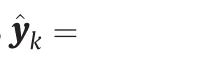
Now we examine the disturbance rejection performance of the proposed MPC.Here we consider three unmeasured disturbances as shown in Fig.7.We also use the same parameters as before.Moreover,the disturbance rejection performance is shown in Figs.8–10.

Fig.7.Unmeasured disturbances for the disturbance rejection test in the distillation column.

Fig.8.Disturbance rejection performance of MPC using different disturbance models for the distillation column(overhead composition).

Fig.9.Disturbance rejection performance of MPC using different disturbance models for the distillation column(bottom composition).

Fig.10.Disturbance rejection performance of MPC using different disturbance models for the distillation column(manipulated variables).

The output disturbance model gives the worst performance from Figs.8–10.This type of disturbance model has been criticized by many authors[13,27].As shown in Section 2.1,the input disturbance model can cover model mismatch and unmeasured disturbances,thus,the input disturbance model often provides better performance than the output disturbance model.Here we can see that the input disturbance model based MPC and the proposed MPC have a similar rejection performance,but the proposed approach is slightly better.From this test,we can see that the proposed MPC is adequate for handling model mismatch and unmeasured disturbances for non-linear plants.

7.Conclusions

The use of optimal filters for linear offset-free MPC is discussed in this study.As distinct from existing approaches,the proposed method does not require any assumptions about the dynamics of disturbances,and disturbances are allowed to have arbitrary statistics.As a result,disturbance modeling requires less work and is more practical to implement.Moreover,we show that the proposed MPC can achieve offset-free control.Tracking performance using this approach is often comparable with the KF based approaches,and the proposed approach performs better in rejecting unmeasured disturbances,which is often more important than the tracking performance in many implementations.

[1]B.W.Bequette,Non-linear model predictive control:A personal retrospective,Can.J.Chem.Eng.85(4)(2007)408–415.

[2]S.J.Qin,T.A.Badgwell,A survey of industrial model predictive control technology,Control.Eng.Pract.11(7)(2003)733–764.

[3]T.A.Badgwell,K.R.Muske,Disturbance model design for linear model predictive control,Proceedings of the American Control Conference,Anchorage,2002,pp.1621–1625.

[4]U.Maeder,Borrelli,M.Morari,Linear offset-free model predictive control,Automatica45(10)(2009)2214–2222.

[5]M.Morari,U.Maeder,Nonlinear offset-free model predictive control,Automatica48(9)(2012)2059–2067.

[6]K.R.Muske,T.A.Badgwell,Disturbance modeling for offset-free linear model predictive control,J.Process Control12(5)(2002)617–632.

[7]G.Pannocchia,A.Bemporad,Combined design of disturbance model and observer for offset-free model predictive control,IEEE Trans.Autom.Control52(6)(2007)1048–1053.

[8]G.Pannocchia,E.C.Kerrigan,Offset-free receding horizon control of constrained linear systems,AIChE J.51(12)(2005)3134–3146.

[9]G.Pannocchia,J.B.Rawlings,Disturbance models for offset-free model predictive control,AIChE J.49(2)(2003)426–437.

[10]M.R.Rajamani,J.B.Rawlings,Estimation of the disturbance structure from data using semidefinite programming and optimal weighting,Automatica45(1)(2009)142–148.

[11]B.J.Odelson,M.R.Rajamani,J.B.Rawlings,A new autocovariance least-squares method for estimating noise covariances,Automatica42(2)(2006)303–308.

[12]M.R.Rajamani,J.B.Rawlings,S.J.Qin,Achieving state estimation equivalence for misassigned disturbances in offset-free model predictive control,AIChE J.55(2)(2009)396–407.

[13]F.G.Shinskey,Feedback Controllers for the Process Industries,McGraw-Hill Professional,1994.

[14]K.R.Muske,J.B.Rawlings,Model predictive control with linear models,AIChE J.39(2)(1993)262–287.

[15]S.Gillijns,B.De Moor,Unbiased minimum-variance input and state estimation for linear discrete-time systems,Automatica43(1)(2007)111–116.

[16]S.Gillijns,B.De Moor,Unbiased minimum-variance input and state estimation for linear discrete-time systems with direct feedthrough,Automatica43(5)(2007)934–937.

[17]P.K.Kitanidis,Unbiased minimum-variance linear state estimation,Automatica23(6)(1987)775–778.

[18]T.Kailath,A.H.Sayed,B.Hassibi,Linear Estimation,Prentice-Hall,Upper Saddle River,NJ,2000.

[19]Z.Xu,Y.Zhu,K.Han,J.Zhao,J.Qian,A multi-iteration pseudo linear regression method and an adaptive disturbance model for MPC,J.Process Control20(4)(2010)384–395.

[20]M.Darouach,M.Zasadzinski,Unbiased minimum variance estimation for systems with unknown exogenous inputs,Automatica33(4)(1997)717–719.

[21]H.Z.Fang,R.A.de Callafon,On the asymptotic stability of minimum-variance unbiased input and state estimation,Automatica48(12)(2012)3183–3186.

[22]W.Kerwin,J.Prince,On the optimality of recursive unbiased state estimation with unknown inputs,Automatica36(9)(2000)1381–1383.

[23]Y.Cheng,H.Ye,Y.Wang,D.Zhou,Unbiased minimum-variance state estimation for linear systems with unknown input,Automatica45(2)(2009)485–491.

[24]H.Wang,J.Zhao,Z.Xu,Z.Shao,Input and state estimation for linear systems with a rank-de ficient direct feedthrough matrix,ISA Trans.57(2015)57–62.

[25]H.Wang,J.Zhao,Z.Xu,Z.Shao,Model predictive control for Hammerstein systems with unknown input nonlinearities,Ind.Eng.Chem.Res.53(18)(2014)7714–7722.

[26]S.Skogestad,Dynamics and control of distillation columns:A tutorial introduction,Chem.Eng.Res.Des.75(6)(1997)539–562.

[27]P.Lundström,J.H.Lee,M.Morari,S.Skogestad,Limitations of dynamic matrix control,Comput.Chem.Eng.19(4)(1995)409–421.