YIN+Xuefeng+ZHANG+Nan+Stephen+Wang+CHENG+Xiang

Abstract In this paper， the conventional method of establishing spatial channel models （SCMs） based on measurements is extended by including clusters? of? scatterers （CoSs） that exist along propagation paths. The channel models resulted utilizing this new method are applicable for generating channel realizations of reasonable spatial consistency， which is required for designing techniques and systems of the fifth generation wireless communications. The scatterers locations are estimated from channel measurement data obtained using large? scale antenna arrays through the Space? Alternating Generalized Expectation? Maximization （SAGE） algorithm derived under a spherical wavefront assumption. The stochastic properties of CoSs extracted from real measurement data in an indoor environment are presented.

Keywords channel modeling； large?scale antenna array； spatial consistency； space?alternating generalized expectation?maximization （SAGE） algorithm； spherical wavefront

1 Introduction

Channel modeling based on extensive measurement campaigns is important for characterizing wave propagations in real environments [1]. High?resolution channel estimation algorithms， such as the Space?Alternating Generalized Expectation?Maximization （SAGE） [2]， [3] and Richters Maximum Likelihood Estimation （RiMAX） algorithms [4]， are widely adopted for processing channel measurement data. These algorithms are derived from generic parametric multipath models under the specular?path assumption [5]， i.e. the dominant components in a channel are contributed by electromagnetic waves propagating along specular paths with planar wavefront when impinging the antenna arrays in the transmitter （Tx） and the receiver （Rx） [2]， [6]， [7]. An individual path can be described with the delay， direction （including azimuth and elevation） of departure （DoD）， direction of arrival （DoA）， complex?valued 2x2 dual?polarization matrix， and non?zero Doppler frequency in the case where the measurement environment is non?static [8]， [9]. By grouping the paths in a channel as clusters [10]， spatial channel models （SCMs） are established based on the statistics of path clusters. Typical SCMs are those specified in 3GPP TR25.996 [11]， the WINNER II SCM?enhanced model [12]， IMT?Advanced models [13]， and COST 2100 models [14]， [15].

Recently， channel modeling for designing the fifth generation （5G） wireless communication techniques and systems has been paid much attention [3]， [16]-[19]. Spatial channels are exploited unprecedentedly in numerous 5G transmission techniques， such as the massive multiple?input multiple?output （MIMO） system using large?scale antenna arrays. The so?called “spatial consistency” property arises as a new characteristics which has not been effectively modeled in the conventional SCMs. Spatial consistency refers to the inherent relationship of channels observed by a user equipment （UE） in consecutive snapshots or drops when the UE moves in a clutter environment [17， Sect. 2.1]. In order to generate channels with reasonable spatial consistency， a 5G channel model needs to take into account the distribution of scatterers in the environment， a property yet considered in the conventional SCM modeling. To construct models of spatial consistency， the project “Mobile and Wireless Communications Enablers for the Twenty?Twenty Information Society （METIS）” has been proposed to include the geometric locations of the scatterers involved in the first and last hops of each path in SCMs [17]. Such a modeling strategy was adopted for establishing the initial map?based ray?tracing model， where the locations of scatterers are predicted by using a simple geometry?based method from the map of an environment. However， the map?based ray?tracing models are too site?specific to generate channel realizations in general cases. It is necessary to build measurement?based models that take into account the scatterers involved along paths estimated through channel sounding in real environments.

Recently， an algorithm of scatterer localization dedicated for MIMO channel sounding was introduced in [20]. This algorithm was derived under a spherical wavefront assumption and applicable for estimating the scatterers locations along propagation paths. More specifically， this algorithm estimates two more distance parameters in addition to the conventional DoD， DoA， delay and Doppler frequency. These new parameters are the distance between the center of the Tx antenna array to the scatterer in the first hop， and the distance between the center of the Rx antenna array to the scatterer in the last hop of a path. The estimates of these distance parameters can be used together with the DoD and DoA to determine the location of the scatterers involved in the first and last hops of the path respectively. Experimental results illustrated in [20] clearly demonstrate the effectiveness of this algorithm applied to processing measurement data collected using large?scale antenna arrays.

In this paper， we illustrate for the first time， an example of establishing channel models involving cluster of scatterers. We adapt the algorithm derived in [20] for estimating the scatterers locations from single?input multiple?output （SIMO） channel measurements. A large?scale antenna array of 121 elements is used in the receiver side. The clusters of scatterers （CoSs） are extracted and their statistical properties are discussed. This knowledge can be incorporated into the frameworks of SCMs to associate each group of paths with two sets of scatterers located respectively in the first and last hops of the paths. The novelty of this work lies in the following aspects： 1） a new framework of SCMs for reproducing spatial?consistency by including the statistics of CoSs； and 2） an experimental example illustrating the procedure of establishing the CoS?included channel models. The enhanced SCMs resulted are applicable of generating non?stationary channel realizations for many 5G propagation scenarios， such as in the cases of massive MIMO， and of device to device communications with link ends surrounded by scatterers in their proximity.

The rest of this paper is organized as follows. Section 2 brie?y reviews the scatterer localization algorithm derived based on the spherical wavefront assumption. In Section 3， the modeling procedure of including CoSs into SCMs is introduced. Section 4 elaborates the behavior of CoSs extracted from real measurements using a large?scale Rx antenna array in indoor environments. Finally， conclusive remarks are addressed in Section 5.

2 Spherical?Wavefront?Based Scatterer Localization Algorithm

The planar wave assumption has been widely used for deriving high?resolution channel parameter estimation algorithms. This assumption is only valid when the scatterer deviates from an antenna array larger than the Rayleigh distance d Rayleigh=2D 2/[λ]， where D in meters is the aperture of the array and [λ] represents the wavelength of the carrier [21， Chapter 2.2.3]. In the scenarios where an antenna array has a sufficiently large aperture， the distance from the array to a scatterer may be less than d Rayleigh. As a result， the planar wavefront assumption is inappropriate because the wavefront observed at the locations of individual antennas is non?uniform.

Fig. 1 illustrates a diagram of a wave incident to the Rx array when the scatterer that interacts with the wave deviates from the array center with a distance less than d Rayleigh. It should be noticed that the planar array plotted in Fig. 1 is only used as an example. The antenna array has various configurations， such as spherical or cubic. The analysis in the following is conducted regardless of the exact shape of the array. It is obvious from Fig. 1 that when the scatterer is viewed as a point， the DoA of the ?th path observed by the nth Rx antenna is determined by the antennas location [rRx，n]and the location [sRx，l] of the scatterer involved in the last hop of the path. In another word， the DoAs of the ?th path observed at all Rx antennas coincide with the radial directions of the antenna positions in a spherical coordinate system with the origin located at [sRx，l]. Similar effect can be observed for the Tx antenna array in the case where the scatterer involved in the first hop of a path is so close to the Tx antenna array that the DoD observed at a Tx antenna is determined by the position [rTx，m] of the Tx antenna and the location [sTx，l] of the scatterer. The phenomenon of wave propagating with spherical wavefronts is often observed in the MIMO channel obtained by using large?scale antenna arrays. Since a planar wave can be viewed as a special case of waves with spherical wavefront when the distance between the scatterer emitting the wave and an antenna array is larger than d Rayleigh ， a new spherical?wavefront generic multipath model can be proposed and applied for parameter estimation of all paths in the channel [20]. The advantage of applying spherical?wavefront model is that the estimated parameters of a path can be used to localize the 3?dimensional （3D） locations of scatterers involved in the first and last hops of the paths.

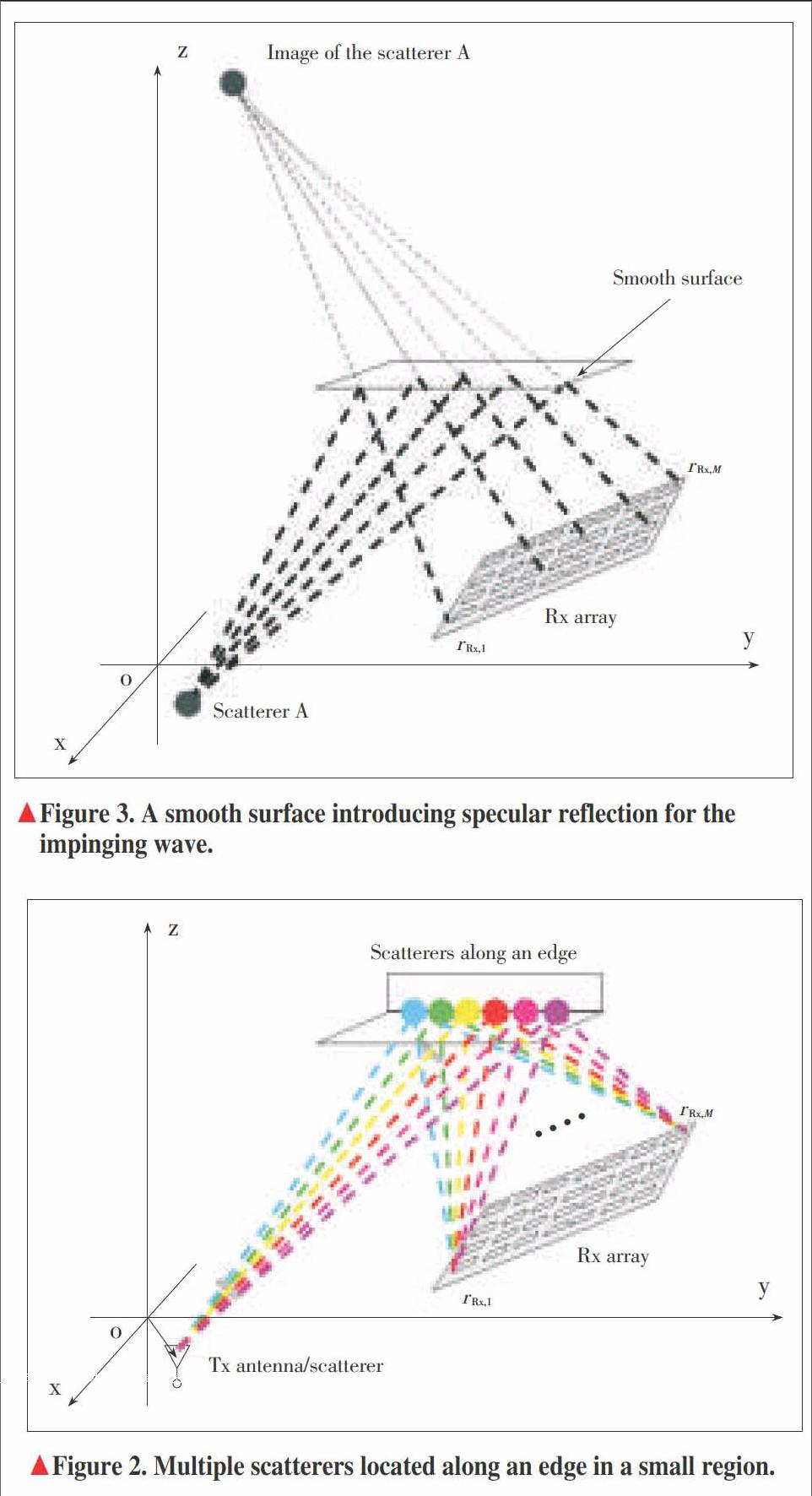
The spherical wavefront assumption relies on the condition that the scatterer is a point source that has infinitesimal small volume. Thus， localization of a scatterer by using parameter estimates obtained under a spherical wavefront is accurate in the case where the physical extent of the scatterer is sufficiently small. However， this is not usually the case in reality. For example， in the scenario where scatterers are spaced closely along an edge as depicted in Fig. 2， due to the limited resolution of the measurement system in both direction and range [22]， it is difficult to resolve these scatterers individually. Thus， the estimated 3D?location of a scatterer under the spherical wavefront assumption may not correspond to the exact location of any of these scatterers. Furthermore， the estimation result could be varying from snapshot to snapshot if the measurements involve random variations of the environment. In the case where the estimated locations of scatterers are close enough， they can be grouped as a CoS and used to describe the distribution of the scatterers along the paths which exhibit similar parameters.

It is worth mentioning that in the case where the true scatterers involved in the first or last hop of a path are located on a smooth surface where specular reflections occur， the localization of a scatterer under the spherical wavefront assumption can be erroneous significantly. Fig. 3 illustrates an example of such a scenario， where every antenna in the Rx array receives the wave reflected by different points on the smooth surface. The estimated 3D location of the scatterer under the spherical wavefront assumption corresponds to the image of the point scatterer with the smooth surface being the mirror. Although the scatterer localization does not provide correct results in such a case， from propagation point of view， the estimated scatterer still provides the contribution equivalent with the true scatterer to the propagation channel. Thus， the CoS formed by the estimated image?scatterers remains important for being considered in channel characterization.

3 SCMs Enhanced by Incorporating CoSs

The positions of scatterers in an environment can be used to predict channel characteristics via ray?tracing [23] or graph?modeling [24]. Similarly， the spatial consistency of channels observed in consecutive snapshots when a UE moves， or the non?stationarity of channel observed from different antennas in massive MIMO scenarios， can be reproduced based on the distribution of scatterers in the environment and their relationships with the propagation paths. In order to generate non?stationary channels with reasonable spatial consistency， the conventional SCMs established with multipath clusters need to incorporate the stochastic characteristics of the scatterers， or CoSs in the first and last hops of paths.

Parameterizing CoS?incorporated SCMs requires localization of the scatterers along multipath. This cannot be effectively performed through conventional MIMO channel measurements that adopt antenna arrays with small apertures， usually less than 3 to 4λ [10， Ch. 9.2]. In many recently conducted measurement campaigns for massive MIMO channel characterization [25]， [26]， large?scale antenna arrays with apertures about dozens of wavelengths are applied. This facilitates the usage of spherical?wavefront estimation algorithms， like that proposed in [20] for extracting the locations of the scatterers， and then incorporates the characteristics of CoSs to SCMs. Some proposals are raised in the following for the exact procedure of including the stochastic behaviors of CoSs into SCMs.

The procedure of establishing an SCM incorporating the characteristics of CoSs is similar with that adopted for generating the standard SCMs [10]， [12]. First， the measurement campaigns that make use of large?scale antenna arrays are conducted. In order to create sufficient randomness in the observations， the scatterers in the measurement environment need to be slightly moved in small ranges in measurement snapshots. Then， the measurement data is processed by using the channel parameter estimation algorithm derived under the spherical wavefront assumption， e.g. the SAGE algorithm [20]. The estimated paths are then clustered based on the parameter estimates that include the conventional geometrical parameters and the distances from the center of Tx array and of Rx array to the scatterers involved in the first and last hops of the path as well. Once the multipath clusters are obtained， the locations of the scatterers for the paths assigned in the same cluster are calculated， and the CoSs involved in the first and last hops of paths respectively are obtained. Based on the characteristics of a large number of estimated CoSs extracted from measurement data， the statistical parameters characterizing the stochastic behaviors of the first?hop and last?hop CoSs， e.g. the 3D extent of CoS and the distributions of scatterers in CoS， are calculated and included as parts of the CoS?incorporated SCMs.

When using the CoS?incorporated SCMs to create random channel realizations， the clusters of paths are first generated randomly. For a cluster， the values of distances between the center of the Tx antenna array and scatterers involved in the first hops of these paths are then generated based on the statistics of the first?hop CoSs. By assigning these distances to the paths in the cluster randomly， the positions of the scatterers in the first hops of paths can be calculated. Similar approaches can be applied to find the positions of the scatterers involved in the last hops of the paths. When the UE moves， or different Tx or Rx antennas in a large?scale array are selected， the corresponding channel is calculated based on the path parameters updated with the new positions of the UE， or the positions of the Tx and Rx antennas in the array respectively.

4 Experimental Results for Characteristics of CoSs

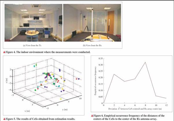
Recently， a measurement campaign for characterizing CoSs has been conducted in an office environment in Toshiba Research Europe ltd.， Bristol， UK. The Toshiba Medav ultra?wide?band （UWB） sliding?correlator channel sounder was applied in the measurements. A SIMO configuration was considered with the Tx equipped with a UWB biconical omnidirectional antenna and the Rx with a 121?element virtual planar antenna array. The sounding signal is generated by using a pseudo?noise m?sequence of 4095 chips， with bandwidth B = 500 MHz and center frequency of 9.5 GHz. The Rx antenna is an omni?directional biconical antenna， which is attached to an extendible fiberglass mast mounted with the movable part of a high?accuracy positioner. The Rx antenna moves along the vertices of 11 × 11 grids to form a virtual antenna array with positioning errors less than 1.2 μm. Each grid is square with edge on one side equal to half the wavelength of the wave with carrier frequency of 9.5 GHz. The vibration caused by relocating the antenna is minimized by calibrating the acceleration and de?acceleration of the motors. After the positioner reaches the desired location， the sounder waits for an additional period of approximately 1 s before measuring. This delay allows any residual vibration to dissipate before capturing CIRs. During the measurements， the environment was kept stationary， the Tx antenna was fixed with height of 1.2 m above the office floor， and the virtual Rx antenna array was located in a horizontal plane which is 1.8 m above the floor.

The measurements were conducted in a room which has the dropped ceiling made of polystyrene faux tile. The floor is a metallic structure covered with carpet tiles. The room has two glass walls， two slat walls， and some office furniture including metallic bench desks and shelves. Fig. 4a illustrates a photograph of the Rx antenna and the positioner in the office， and Fig. 4b shows the photograph of both the Tx and the Rx antennas.

The SAGE algorithm derived in [20] was adapted to the SIMO case considered here. Thus， only the scatterers involved in the last hops of paths can be localized. Furthermore， as the Rx array is located horizontally， the estimation algorithm cannot distinguish whether the waves arrive above or below the plane. In such a case， the estimation range of the elevation of arrival （EoA） is limited to [[90o， 180o]]， i.e. below the array plane. However， it is likely that the paths with true EoA within [[0o， 90o]] are estimated with an EoA symmetric to the true angle with respect to the array plane. The azimuth of arrival estimation range is set to [[-180o， 180o]]. The number L of paths to be estimated is set to 40. It should be noticed that the number of paths can be estimated by applying the Akaike Information Criterion or Minimum Length Description principle [27]. In this preliminary study， we choose to set a large value for L as we usually did in many other works on high?resolution path parameter estimation [2]， [28]. Furthermore， only vertical polarization is considered for estimating the complex attenuations of paths as both Tx and Rx antennas are vertically polarized in the measurements.

Since the SAGE algorithm is applied to estimate L = 40 paths per measurement snapshot， from totally 10 measurement snapshots， we obtain the parameter estimates of 400 paths. During these measurement snapshots， the locations of the Tx antenna and Rx array are kept ?xed， and the environment is unchanged. The randomness in each snapshot is generated by the thermal noise in the measurement equipment. Strictly speaking， the randomness should be generated by slightly changing the environment. A clustering algorithm similar to that introduced in [29] is applied to gather the paths as clusters. Totally 53 CoSs are found. Fig. 5 depicts the locations of scatterers calculated based on the multipath parameter estimates. The spots plotted with same color and same legend marks in Fig. 5 represent the scatterers in the same CoS. These CoSs may not correspond exactly to the true scatterers involved in the last hops of paths due to specular re?ections caused by smooth surfaces existing in the environment， as discussed in Section 2. Thus， it is possible that the distance between a CoS and the Rx array is larger than the physical size of the office where the measurements were conducted. From channel modeling point of view， all the CoSs extracted from the data need to be considered for constructing the stochastic channel model regardless whether the location of an estimated CoS coincides with real scatterers in the environment.

Based on the parameter estimates obtained from multiple snap?shots， the so?called inter?and intra?CoS statistical properties are extracted. The inter?CoS property is referred to as the distribution of the CoSs centroid in a 3D coordinate system. In our case where the sounding signal has 500 MHz bandwidth and center frequency of 9.5 GHz， the estimated CoSs involved in the last hops of paths are distributed within the 3D volume of 15 m ×15 m ×6 m. It is obvious that these dimensions are larger than the extents of the office. We postulate that this is because some CoSs are actually the images of real scatterers in the office due to reflections on the smooth walls.

Another inter?CoS property investigated is the empirical distribution of the distance [d] between the CoS centroid and the center of Rx antenna array. Fig. 6 illustrates the empirical occurrence frequency （EOF） of the distance[ d]. Fig. 6 shows that [d] is distributed with two local maxima located at 2 m and 8 m respectively. This， according to our conjecture， is due to the reason that some scatterers in the environment exist on the ceiling and around the positioner in the vicinity of the Rx array and others are mainly distributed on the outskirts of the office. The former scatterers create the concentration of [d] around 2 m， and the latter lead to the higher occurrence frequency at 8 m. It is worth mentioning that the EOF of [d] observed in these measurements seem to justify the assumption adopted in some channel simulations based on sum?of?sinusoids （SoS）， i.e. the scatterers are distributed along multiple rings centered at the ends of a communication link [30]， [31].

An intra?CoS property considered here is the average empirical EOF of the deviation [d] of the scatterers in a cluster from the centroid of the cluster. Fig. 7 depicts the empirical EOFs of [d ]obtained in two scenarios. The probability density function （PDF） of a Laplacian distribution ?tted to the empirical data is also demonstrated in Fig. 7. It can be observed that the EOF graph is symmetric with respect to [d=0] m. The Laplacian PDF with position parameter [μ=0] m and scaling parameter [b=3.24] exhibits certain deviations from the EoF. We postulate that this is because of the insuf?cient number of samples collected in the study. From Fig. 7 we conclude that the scatterers in a CoS are distributed symmetrically with respect to the CoSs centroid with standard deviation of [2b≈4]cm in the of?ce environment considered.

5 Conclusions

In this paper， a new strategy of incorporating the locations of scatterers into SCM was proposed which is applicable provided the channel measurements are conducted with large?scale antenna arrays. In this scheme， a spherical wavefront parameter estimation algorithm is adopted to extract the distance from the center of transmitting antenna array to the scatterers involved in the first hop of the path， and the distance from the center of receiving antenna array to the scatterers involved in the last hop of the path. These two distance parameters together with direction of departure and direction of arrival can be used to localize scatterers at the first and last hops of the path respectively. The SCM incorporating the statistical characteristics of CoSs is applicable for generating channel realizations in multiple drops with demanded spatial consistency when an user equipment moves， or for non?stationary spatial channels observed through different antennas in massive MIMO scenarios. Channel measurement data were collected by using a Toshiba ultra?wideband sounder equipped an 11×11 virtual receiver antenna array and sounding signals of 500 MHz bandwidth at center frequency of 9.5 GHz. These data have been applied to illustrate the modeling procedure for the characteristics of CoSs. Based on the parameter estimates obtained from multiple snapshots， the inter?CoS and intra?CoS statistical properties were extracted， including the distribution of the centroid of CoSs， and the distribution of scatterers in individual CoSs for the indoor environment considered in the measurements. This work can supply significant guidelines for conducting measurements and modeling channels aiming at reproducing the spatial?consistency by including the statistical information of environments.

References

[1] E. Bonek， M. Herdin， W. Weichselberger， and H. ?zcelik， “MIMO—study propagation first！” in 3rd IEEE International Symposium on Signal Processing and Information Technology （ISSPIT）， Darmstadt， Germany， Dec. 2003. pp. 150-153， doi： 10.1109/ISSPIT.2003.1341082.

[2] B. H. Fleury， M. Tschudin， R. Heddergott， D. Dahlhaus， and K. L. Pedersen， “Channel parameter estimation in mobile radio environments using the SAGE algorithm，” IEEE Journal of Selected Areas in Communications， vol. 17， no. 3， pp. 434-450， Mar. 1999. doi： 10.1109/49.753729.

[3] X. Yin， C. Ling， and M. Kim， “Experimental multipath?cluster characteristics of 28?GHz propagation channel，” IEEE Access， vol. 3， pp. 3138-3150， 2016. doi：10.1109/ACCESS.2016.2517400.

[4] A. Richter， M. Landmann， and R. S. Thom?， “Maximum likelihood channel parameter estimation from multidimensional channel sounding measurements，” in 57th IEEE Vehicular Technology Conference （VTC）， Jeju， South Korea， 2003， pp. 1056-1060. doi： 10.1109/VETECS.2003.1207788.

[5] J. Fuhl， J.?P. Rossi， and E. Bonek， “High?resolution 3?D direction?of?arrival determination for urban mobile radio，” IEEE Transactions on Antennas and Propagation， vol. 45， no. 4， pp. 672 -682， 1997. doi： 10.1109/8.564093.

[6] A. Paulraj， R. Roy， and T. Kailath， “Estimation of signal parameters via rotational invariance techniques—ESPRIT，” in 19th Asilomar Conference on Circuits， Systems and Computers， Pacific Grove， USA， Nov. 1985， pp. 83-89. doi： 10.1109/ACSSC.1985.671426.

[7] R. Roy and T. Kailath， “ESPRIT—estimation of signal parameters via rotational invariance techniques，” IEEE Transactions on Acoustics， Speech， and Signal Processing， vol. 37， no. 7， pp. 984-995， Jul. 1989. doi： 10.1109/29.32276.

[8] X. Yin， B. H. Fleury， P. Jourdan， and A. Stucki， “Polarization estimation of individual propagation paths using the SAGE algorithm，” in IEEE International Symposium on Personal， Indoor and Mobile Radio Communications （PIMRC）， Beijing， China， Sep. 2003. pp. 1795-1799， doi： 10.1109/PIMRC.2003.1260424.

[9] B. H. Fleury， X. Yin， K. G. Rohbrandt， P. Jourdan， and A. Stucki， “High?resolution bidirection estimation based on the sage algorithm： Experience gathered from field experiments，” in XXVIIth General Assembly of the Int. Union of Radio Scientists （URSI）， Maastricht， Netherlands， vol. 2127， 2002.

[10] N. Czink， “The random?cluster model ?a stochastic MIMO channel model for broadband wireless communication systems of the 3rd generation and beyond，” Ph.D. dissertation， Technische Universitat Wien， Vienna， Austria， FTW Dissertation Series， 2007.

[11] Universal Mobile Telecommunications System （UMTS）；Spacial Channel Model for Multiple Input Multiple Output （MIMO） Simulations， 3GPP TR 25.996 version 8.0.0 Release 8， 2008.

[12] WINNER II Interim Channel Models， IST?4?027756 WINNER D1.1.1 Std.， 2007.

[13] Guidelines for Evaluation of Radio Interface Technologies for IMT?Advanced （12/2009）， ITU?R M.2135?1 Std， 2009.

[14] L. Liu， C. Oestges， J. Poutanen， et al.， “The COST 2100 MIMO channel model，” IEEE Transactions on Wireless Communications， vol. 19， no. 6， pp. 92-99， Dec. 2012. doi： 10.1109/MWC.2012.6393523.

[15] M. Zhu， G. Eriksson， and F. Tufvesson， “The COST 2100 channel model： parameterization and validation based on outdoor MIMO measurements at 300 MHz，” IEEE Transactions on Wireless Communications， vol. PP， no. 99， pp. 1-10， 2013. doi： 10.1109/TWC.2013.010413.120620.

[16] J. Medbo， K. B?rner， K. Haneda， et al.， “Channel Modelling for the Fifth Generation Mobile Communications，”in Eighth European Conference on Antennas and Propagation （EuCAP）， Hague， Holland， Apr. 2014， pp. 1-5. doi： 10.1109/EuCAP.2014.6901730.

[17] T. J?ms?， P. Ky?sti， and K. Kusume， “Deliverable D1.2 Initial channel models based on measurements，” Project Name： Scenarios， requirements and KPIs for 5G mobile and wireless system （METIS） ， Document Number： ICT?317669?METIS/D1.2， Tech. Rep.， 2014. [Online]. Available： www.metis2020.com

[18] Y. Ji， X. Yin， H. Wang， X. Lu， and C. Cao， “Antenna?de?embedded characterization for 13?17 ghz wave propagation in indoor environments，” IEEE Antennas and Wireless Propagation Letters， vol. PP， no. 99， pp. 1-1， 2016. doi： 10.1109/LAWP.2016.2553455.

[19] X. Yin， L. Ouyang， and H. Wang， “Performance comparison of sage and music for channel estimation in direction?scan measurements，” IEEE Access， vol. 4， pp. 1163-1174， 2016. doi： 10.1109/ACCESS.2016.2544341.

[20] J. Chen， S. Wang， and X. Yin， “A spherical?wavefront?based scatterer localization algorithm using large?scale antenna arrays，” IEEE Communications Letters， vol. 20， no. 9， pp. 1796-1799， Sept. 2016. doi： 10.1109/LCOMM.2016.2585478.

[21] C. A. Balanis， Antenna Theory Analysis and Design， 3rd ed. Hoboken， USA： John Wiley & Sons， 2005.

[22] X. Yin and X. Cheng， Propagation Channel Characterization， Parameter Estimation and Modeling for Wireless Communications. Hoboken， USA： John Wiley & Sons， 2016.

[23] V. Degli?Esposti， D. Guiducci， A. deMarsi， P. Azzi， and F. Fuschini， “An advanced field prediction model including diffuse scattering，” IEEE Transactions on Antennas and Propagation， vol. 52， no. 7， pp. 1717-1728， 2004. doi： 10.1109/TAP.2004.831299.

[24] T. Pedersen， G. Steinbock， and B. Fleury， “Modeling of reverberant radio channels using propagation graphs，” IEEE Transactions on Antennas and Propagation， vol. 60， no. 12， pp. 5978-5988， 2012. doi： 10.1109/TAP.2012.2214192.

[25] X. Gao， F. Tufvesson， O. Edfors， and F. Rusek， “Measured propagation characteristics for very?large MIMO at 2.6 GHz，” in IEEE 46th Asilomar Conference on Signals， Systems and Computers （ASILOMAR）， Pacific Grove， USA， 2012， pp. 295-299. doi： 10.1109/ACSSC.2012.6489010.

[26] X. Gao， F. Tufvesson， and O. Edfors， “Massive MIMO channels?Measurements and models，” in IEEE Asilomar Conference on Signals， Systems and Computers， Pacific Grove， USA， 2013， pp. 280-284. doi： 10.1109/ACSSC.2013.6810277.

[27] H. Akaike， “A new look at the statistical model identification，” IEEE Transactions on Automatic Control， vol. AC?19， no. 6， pp. 716-723， Dec. 1974. doi： 10.1109/TAC.1974.1100705.

[28] C.?C. Chong， C.?M. Tan， D. Laurenson， et al.， “A new statistical wideband spatio?temporal channel model for 5?GHz band WLAN systems，” IEEE Journal on Selected Areas in Communications， vol. 21， no. 2， pp. 139-150， 2003. doi： 10.1109/JSAC.2002.807347.

[29] N. Czink， P. Cera， J. Salo， et al.， “A framework for automatic clustering of parametric MIMO channel data including path powers，” in IEEE 64th Vehicular Technology Conference， Montreal， Canada， Sept. 2006， pp. 1-5. doi： 10.1109/VTCF.2006.35.

[30] X. Cheng， C.?X. Wang， H. Wang， et al.， “Cooperative MIMO channel modeling and multi?link spatial correlation properties，” IEEE Journal on Selected Areas in Communications， vol. 30， no. 2， pp. 388-396， Feb. 2012. doi： 10.1109/JSAC.2012.120218.

[31] Y. Wang and A. Zoubir， “Some new techniques of localization of spatially distributed sources，” in Forty?First IEEE Asilomar Conference on Signals， Systems and Computers （ACSSC）， Pacific Grove， USA， 2007， pp. 1807-1811. doi： 10.1109/ACSSC.2007.4487546.

Manuscript received： 2016?11?27