ZHANG+Ping+CHEN+Jianqiao+TANG+Tian

Abstract Massive multiple?input multiple?output （MIMO） emerges as one of the most promising technologies for 5G mobile communication systems. Compared to the conventional MIMO channel models， channel researches and measurements show that significant non?stationary properties rise in massive MIMO channels. Therefore， an accurate channel model is indispensable for the sake of massive MIMO system design and performance evaluation. This article presents an overview of methods of modeling non?stationary properties on both the array and time axes， which are mainly divided into two major categories： birth?death （BD） process and cluster visibility region （VR） method. The main concepts and theories are described， together with useful implementation guidelines. In conclusion， a comparison between these two methods is made.

Keywords birth?death process； cluster visibility region method； massive MIMO channel model； non?stationary properties

1 Introduction

Massive multiple?input multiple?output （MIMO） systems， which are equipped with tens or even hundreds of antennas， have been proposed to meet the increasing traffic demand of the future wireless communication systems. Compared to conventional MIMO systems， massive MIMO systems are able to substantially improve capacity， link reliability， energy efficiency and spectral efficiency [1]-[4]. For the sake of MIMO system design and performance evaluation， it is indispensable to develop accurate and efficient small?scale fading channel models. Generally， there are three generic approaches for conventional MIMO channel modeling， namely the stochastic model， deterministic?based model and geometry?based stochastic model （GBSM）. The GBSM has been widely used as an efficient method to simulate the wireless propagation channels， because it generates the location of scatterers according to a certain probability distribution rather than specific channel environment. So far， many standardized GBSMs are proposed [5]-[7]. However， according to the channel measurements [8]， [9]， new characteristics of the massive systems make the conventional MIMO channel models not be effective to be applied in massive MIMO channels directly.

Non?stationary property is one of the new characteristics that makes massive MIMO channels different from conventional ones. Non?stationary property generally includes two aspects： angle of arrival （AOA） shifts at the receiver side and dynamic properties of clusters on both the array and time axes. AOA shifts can be described completely through spherical wave?front assumption according to geometrical relationships among transmitter， receiver and clusters [10]. This article does not focus on this aspect. Dynamic properties of clusters on both the array and time axes generally refer to the facts that each antenna at different physical location has different cluster sets and the location of cluster is changing over time. This property is mainly described through birth?death （BD） process and cluster visibility region （VR） method.

The BD process was first investigated to model the non?stationary properties of clusters on the time axis only [11]-[14]. After this property was observed on the large antenna array [8]， [9]， i.e.， appearance and disappearance of clusters can occur on the array axis， the BD process was extended to the antenna array [15]-[17]. The authors in [15] proposed a 2D ellipse model that describes wide?band massive MIMO channels by many con?focal ellipses. Similarly， a 2D multi?ring channel model with the same center for massive MIMO was proposed in [16]. For both of them， the geometrical relationships related to the delays of multi?path components （MPCs） are assumed to mimic the distribution of clusters. In [17]， a 3D twin?cluster model was proposed， where a cluster was divided into two representations of itself （one at the transmitter and the other at the receiver）. Then the complicated scattering environment was abstracted by a virtual link between the two representations of this cluster. Although the descriptions of geometrical relationships are different in these modeling approaches， the methods of modeling non?stationary properties of clusters on both the array and time axes are all based on the BD process.

The cluster VR method models the non?stationary properties of clusters from the cluster perspective. VR is typically assigned to the cluster in such a way that when an terminal enters a VR， the cluster assigned to this VR is active （contributes to the impulse response）. The cluster VR method was investigated on the time axis at first [18]， and after the non?stationary properties of clusters on the large antenna array in massive MIMO was observed， it was extended [19]-[21]. In [19]， a 3D two?cylinder regular?shaped GBSM for non?isotropic scattering massive MIMO channels was proposed. Non?stationary properties of clusters on the array axis were described by using a virtual sphere. In [20] and [21]， the concept of VR in COST 2100 channel model was extended. In [20]， the cluster VR was divided into two categories： the observed VR and the true VR. The cumulative distribution function （CDF） of the observed VR size could be written as a function of the probability density function （PDF） of the true VR size. On the other hand， the distribution of the true VR lengths could be obtained based on measurements. In [21]， cluster VR on the array axis was characterized by the partially visible clusters and wholly visible clusters. Therefore， when using the cluster VR method to describe non?stationary properties of clusters， the definition of VR is most important.

This article aims to give a concise overview of methods of modeling non?stationary properties of clusters for massive MIMO， which mainly include two categories： BD process and cluster VR method. For the BD process， because of uniform modeling approach， a main flow chart that describes non?stationary properties of clusters on both the array and time axes is given. For the cluster VR method， some typical representatives of defining VR in different modeling approach are reviewed. A brief comparison of these two different methods is also given.

2 Birth?Death Process

The BD process is widely investigated to describe non?stationary properties of clusters on both the array and time axes in massive MIMO channel model. In this process， cluster evolution along array and time axes are calculated separately. The main flow of BD process is presented below.

Let [Ntotal] be the total number of clusters that are observable to at least one transmit antenna and one receive antenna. The value of [Ntotal] can be expressed as

where the operator card[?]denotes the cardinality of a set， [MT] and [MR] denote the number of antenna elements at the transmitter and receiver， respectively， and [CTl（t）（CRk（t））] denotes the cluster set in which clusters are observable to the [l]? th transmit antenna （the [k]?th receive antenna ） at time instant [t]. Then， a cluster is observable to the [l]? th transmit antenna and the [k]? th receive antenna if and only if this cluster is in the set [{CTl（t）?CRk（t）}]. Cluster evolution on both the array and time axes determine cluster sets in [CTl（t）]and [CRk（t）].

Cluster evolution on the array axis is operated first. We assume the initial number of clusters [N]and the initial cluster sets of the 1?st transmit and receive antenna [CT1={cTx：x=] [1，2，...，N}]and [CR1={cRx：x=1，2，...，N}] at the initial time instant [t] are given， where [cTx] and [cRx] are two representations of Clusterx， the subscript [x] represents the [x]?th cluster in cluster sets. Then， these clusters in cluster sets [CT1] and [CR1] evolve according to BD process on the array axis to recursively generate the cluster sets of the rest of antennas at the transmitter and receiver at the initial time instant [t]， which can be expressed as

After cluster evolution on the time axis， as （5）-（7） show， all clusters can be categorized as survived clusters or newly generated clusters. For the survived cluster， channel parameters should be updated from [tm] to [tm+1] according to the geometrical relationships. For the newly generated cluster， it is first attached to one transmit antenna element randomly， and then evolves along transmit antenna array to determine whether it can be observed based on the survival probabilities [PTsurvival] on the array axis. The same judge process applies to the receive antenna array too. Finally， the cluster is added to antenna cluster sets if and only if it survives at both the transmitter and receiver side. The main flow of cluster evolution on both array and time axes based on the BD process is given in Fig. 2.

3 Cluster Visibility Region Method

The cluster VR method describes non?stationary properties of clusters on both the array and time axes from the cluster perspective. In the exsiting channel models， different definitions of VR determine the methods of modeling cluster evolution. Therefore， the descriptions of VR in some representative channel models are reviewed separately.

3.1 COST 2100 Channel Model

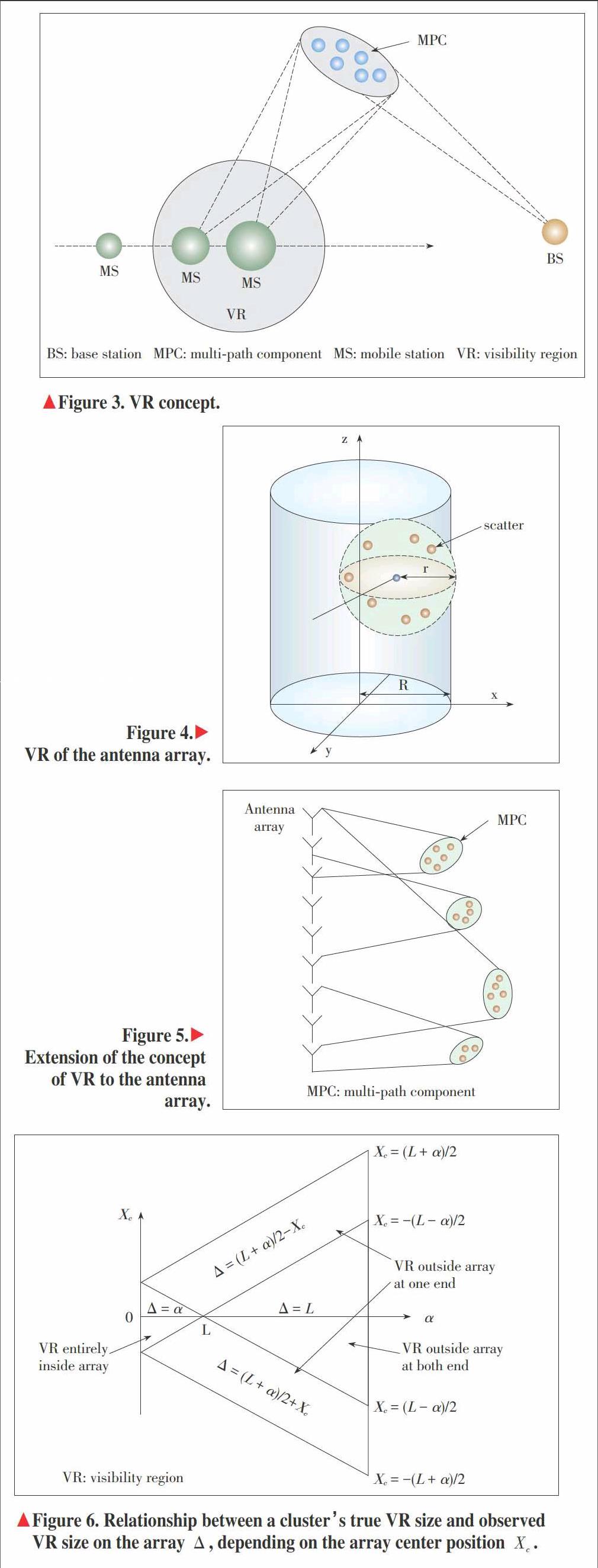
In the COST2100 channel model， the cluster VR method is used to describe cluster evolution on the time axis. Specifically， clusters are divided into three categories： local clusters， single?bounce clusters and multiple?bounce clusters. VR confines the cluster activity within a limited geographical area. A cluster is depicted as an ellipsoid as viewed from mobile stations （MS） and from base stations （BS）， and the size of the circle around the MS represents the visibility level of the cluster to the BS?MS channel， as illustrated in Fig. 3. After the MS moves into the VR， it receives signals scattered by the related cluster. As it moves towards the VR center， the cluster smoothly increases its visibility. The visibility is accounted mathematically by a VR gain， which grows form 0 to 1 upon entrance of the VR. By employing the VR size and the VR gain， cluster evolution at the receiver side can be described in the COST2100 channel model. Eventually， the channel impulse response （CIR） is obtained by the superposition of the MPCs from all active clusters determined by the position of the terminal. Additionally， parameterization and validation of the COST2100 channel model are given in [23] and [24] based on measurements.

3.2 3D TwoCylinder Channel Model

The 3D two?cylinder channel model extends the concept of VR to the antenna array. All the scatterers are distributed on the surface of a cylinder as equivalent， and each antenna has its own visible area of scatterers by using a virtual sphere， where the radius is [r] and the center is the antenna element itself. In this case， scatterers on the surface of the cylinder can be seen by an antenna element only if the distance between them is less than [r]， as shown in Fig. 4. The radius [r]of the virtual sphere can be calculated according to the distance between two antenna elements and the correlation of their channel impulse responses. Furthermore， channel impulse responses are affected by the distribution of scatterers. If the distance is [λ2]， correlation coefficient is 0.9， and scatterers are uniformly distributed on the surface of the cylinder， whose radius is [R]， the [r] can be expressed in terms of [R] as

3.3 Channel Model Based on Extended Concepts of VR

The channel models proposed in [20] and [21] extend the concept of VR in COST2100 channel model to the antenna array. We take the extension in [20] as an example. In [20]， VR size and visibility gain are discussed based on measurements. As shown in Fig. 5， the VR size of some clusters is entirely inside the array， while that of other clusters overlaps one or both ends of the antenna array. For the former case， the observed size of VR on the antenna array is the clusters true VR size， while for the latter case， the true VR size may be much larger than what is observed on the antenna array.

As a result， VR size should be described in two stages. First， the relationship between the observed VR size and the true VR size is determined， as illustrated in Fig. 6. The CDF of the observed VR size [KΔ（y）] can be written as a function of PDF of the true VR size [fα（ν）]， and it can be expressed aswhere [L] is the length of the array， and [Δ0] is the smallest observation of the VR size on the array due to measurement data processing. Second， the particular distribution of the true VR size is calculated through the maximum likelihood estimate （MLE） approach based on the measurements. Finally， the VR size can be calculated.

4 Conclusions

In this article， we review methods of modeling non?stationary properties of clusters on both the array and time axes， namely BD process and cluster VR method. The main flow of BD process is given， and different definitions of VR in some representative channel models are reviewed. Based on mathematical derivation， the theory of BD process is more mature and complete， and its accuracy has been proved by lots of researches. However， it is too complex and lacks of intuitive geometric characteristics between clusters and the antenna array. On the other hand， the cluster VR method pays more attention to geometrical distribution of clusters， which makes it more natural to be integrated into the channel model based on stochastic geometry. However， further study is necessary to obtain the complete information of VR. From our point of view， a better scheme of modeling cluster evolution is to combine these two methods together. This scheme can reduce the complexity of modeling， and also reflect the geometrical characteristics of the channel.

References

[1] D. Gesbert， M. Shafi， D. Shiu， et al.， “From theory to practice： an overview of MIMO space?time coded wireless systems，” IEEE Journal on Selected Areas in Communications， vol. 21， no. 3， pp. 281-302， Apr. 2003. doi： 10.1109/JSAC.2003.809458.

[2] E. G. Larsson， F. Tufvesson， O. Edfors， et al.， “Massive MIMO for next generation wireless systems，” IEEE Communications Magazine， vol. 52， no. 2， pp. 186-195， Feb. 2014. doi： 10.1109/MCOM.2014.6736761.

[3] F. Rusek， D. Persson， B. K. Lau， et al.， “Scaling up MIMO： opportunities and challenges with very large arrays，” IEEE Signal Processing Magazine， vol. 30， no. 1， pp. 40-60， Jan. 2012. doi： 10.1109/MSP.2011.2178495.

[4] L. Lu， G. Y. Li， A. L. Swindlehurst， et al.， “An overview of massive MIMO benefits and challenges，” IEEE Journal of Selected Topics in Signal Processing， vol. 8， no. 5， pp. 742-758， Oct. 2014. doi： 10.1109/JSTSP.2014.2317671.

[5] Spatial Channel Model for Multiple Input Multiple Output （MIMO） Simulations， 3GPP TR 25.996 version 12.0.0 Release 12， 2014.

[6] P. Ky?sti， J. Meinil?， L. Hentil?， et al.， “WINNER II channel models part II radio channel measurement and analysis results，” IST?4?027756 WINNER II D1.1.2 V1.2， 2007.

[7] Guidelines for Evaluation of Radio Interface Technologies for IMT?Advanced， ITU M.2135?0， 2008.

[8] S. Payami and F. Tufvesson， “Channel measurements and analysis for very large array systems at 2.6 GHz，” in Proc. 6th European Conference on Antennas and Propagation， Prague， Czech Republic， Mar. 2012， pp. 433-437.

[9] X. Gao， F. Tufvesson， O. Edfors， et al.， “Measured propagation characteristics for very?large MIMO at 2.6 GHz，” in Proc. 46th Annual Asilomar Conference on Signals， Systems， and Computers， California， USA， Nov. 2012， pp. 295-299.

[10] F. B?hagen， P. Orten， and G. E. ?ien， “On spherical vs. plane wave modeling of line?of?sight MIMO channels，” IEEE Transactions on Communications， vol. 57， no. 3， pp. 841-849， Mar. 2009.

[11] T. Zwick， C. Fischer， D. Didascalou， et al.， “A stochastic spatial channel model based on wave?propagation modeling，” IEEE Journal on Selected Areas in Communications， vol. 18， no. 1， pp. 6-15， Jan. 2000.

[12] T. Zwick， C. Fischer， and W. Wiesbeck， “A stochastic multipath channel model including path directions for indoor environments，” IEEE Journal on Selected Areas in Communications， vol. 20， no. 6， pp. 1178-1192， Aug. 2002.

[13] C. C. Chong， C. M. Tan， D. I. Laurenson， et al.， “A novel wideband dynamic directional indoor channel model based on a Markov process，” IEEE Transactions on Wireless Communications， vol. 4， no. 4， pp. 1539-1552， Jul. 2005. doi： 10.1109/TWC.2005.850341.

[14] F. Babich and G. Lombardi， “A Markov model for the mobile propagation channel，” IEEE Transactions on Vehicular Technology， vol. 48， no. 1， pp. 63-73， Jan. 2000.

[15] S. B. Wu， C. X. Wang， H. Haas， et al.， “A non?stationary wideband channel model for massive MIMO communication systems，” IEEE Transactions on Wireless Communications， vol. 14， no. 3， pp. 1434-1446， 2015.

[16] H. L. Wu， S. Jin， and X. Q. Gao， “Non?stationary multi?ring channel model for massive MIMO systems，” in International Conference on Wireless Communications & Signal Processing （WCSP）， Nanjing， China， 2015， pp.1-6.

[17] S. B. Wu， C. X. Wang， H. Haas， et al.， “A non?stationary 3D wideband twin?cluster model for 5G massive MIMO channels，” IEEE Journal on Selected Areas in Communications， vol. 32， no. 6， pp. 1207-1218， 2014.

[18] L. F. Liu， C. Oestges， J. Poutanen， et al.， “The COST 2100 MIMO channel model，” IEEE Wireless Communications， vol. 19， no. 6， pp. 92-99， Dec. 2012. doi： 10.1109/MWC.2012.6393523.

[19] Y. Xie， B. Li， X. Y. Zuo， et al.， “A 3D geometry?based stochastic model for 5G massive MIMO channels，” in 11th International Conference on Heterogeneous Networking for Quality， Reliability， Security and Robustness （QSHINE）， Taiwan， China， 2015， pp. 216-222.

[20] X. Gao， F. Tufvesson， and O. Edfors， “Massive MIMO channels—measurements and models，” in 2013 Asilomar Conference on Signals， Systems and Computers， Pacific Grove， USA， Nov. 2013， pp. 280-284. doi： 10.1109/ACSSC.2013.6810277.

[21] X. R. Li， S. D. Zhou， E. Bjornson， et al.， “Capacity analysis for spatially non?wide sense stationary uplink massive MIMO systems，” IEEE Transactions on Wireless Communications， vol. 14， no. 12， pp. 7044-7056， 2015.

[22] T. Zwick， C. Fischer， D. Didascalou， and W. Wiesbeck， “A stochastic spatial channel model based on wave?propagation modeling，” IEEE Journal on Selected Areas in Communications， vol. 18， no. 1， pp. 6-15， Jan. 2000.

[23] M. F. Zhu， G. Eriksson， and F. Tufvesson， “The COST 2100 channel model： parameterization and validation based on outdoor MIMO measurements at 300 MHz，” IEEE Transactions on Wireless Communications， vol. 12， no. 2， pp. 888-897， 2013. doi： 10.1109/TWC.2013.010413.120620.

[24] J. Poutanen， K. Haneda， L. F. Liu， et al.， “Parameterization of the COST 2100 MIMO channel model in indoor scenarios，” in Proc. 5th European Conference on Antennas and Propagation （EUCAP）， Rome， Italy， 2011， pp. 3606-3610.

Manuscript received： 2016?11?11