YANG+Mi+HE+Ruisi+AI+Bo+XIONG+Lei+DONG+Honghui+LI+Jianzhi+WANG+Wei+FAN+Wei+QIN+Hongfeng

Abstract The fifth generation （5G） communication has been a hotspot of research in recent years， and both research institutions and industrial enterprises put a lot of interests in 5G communications at some new frequency bands. In this paper， we investigate the radio channels of 5G systems below 6 GHz according to the 5G communication requirements and scenarios. Channel measurements were conducted on the campus of Beijing Jiaotong University， China at two key optional frequency bands below 6 GHz. By using the measured data， we analyzed key channel parameters at 460 MHz and 3.5 GHz， such as power delay profile， path loss exponent， shadow fading， and delay spread. The results are helpful for the 5G communication system design.

Keywords channel measurement； 5G； channel characterization

1 Introduction

In the last decade， public networks have been evolving from voice?centric second?generation systems， e.g.， Global System for Mobile Communications （GSM） with limited capabilities， to fourth?generation （4G） broadband systems that offer higher data rates， e.g.， long?term evolution （LTE） [1]. In recent years， with the rapid development of data services， the fifth generation （5G） communication has attracted high attention both from research institutions and industrial enterprises. According to the IMT-2020 [2]， in some key competencies， 5G needs to support 0.1-1 Gb/s rate， 106 devices/km2 connection density， and below 1 ms end?to?end latency [3].

ITU has suggested a bandwidth for 5G communication systems up to 1490-1810 MHz. The bandwidth of the current plan， however， is only 687 MHZ， which is obviously insufficient. Facing the shortage of spectrum resources shortage， we can use a higher frequency band， or consider other frequency bands below 6 GHz to use the spectrum more efficiently. Since the low frequency band supports a larger propagation distance， it can effectively reduce the number of base stations and decrease the transmission power to save energy.

In the World Radio Communication Conference （WRC） in 2015， eight new frequency bands for International Mobile Telecommunication （IMT） was added in the proposal AI1.1， which are all below 6 GHz， including 470-698 MHz， 1427-1518 MHz， 3300-3400 MHz， 3400-3600 MHz， 3600-3700 MHz， 4800-4990 MHz， etc. At the same time， China also introduced candidate frequency bands to the international standard organizations， and mostly of them are below 6 GHz， e.g.， 3.3-3.6 GHz， 4.4-4.5 GHz and 4.8-4.99 GHz.

If we want to use below 6 GHz frequency bands in 5G communication systems， there are mainly two methods. One is to reuse the existing spectrums， and the other one is to use the new spectrums suggested in WRC 2015. The existing spectrums that can be reused include 800 MHz， 900 MHz， 1.8 GHz and 2.1 GHz. Among the new spectrums， the 3400-3600 MHz band has been considered as the 5G test frequency band， and it is also expected to be the first frequency band for 5G communications in China.

We have done related measurements and achieved some results on campus scenarios at 3.5 GHz [4]. In this paper， we carry out more measurements and analyses， and some rich and more meaningful results are obtained. We also present a channel measurement campaign for campus scenarios performed at two frequency bands （i.e.， 460 MHz and 3.5 GHz）. Furthermore， based on analysis of the measurement data， we present results on key channel parameters in terms of power delay profile， path loss exponent， shadow fading， and delay spread. The results can be used in the 5G communication system design.

The remainder of the paper is organized as follows. Section 2 describes the measurement system and measurement environment. Section 3 presents the measurement results of channel characterizations. Conclusions are drawn in Section 4.

2 Measurement Campaign

We describe our measurement campaign in the light of calibration， measurement system and measurement environment.

2.1 Calibration

2.2 Measurement System

The measurement system is depicted in Fig. 1. Fig. 1a shows the measurement system architecture， including the transmitter， receiver， clock modules， power amplifier and antennas. Fig. 1b shows the transmitter and receiver， which are the core parts of the measurement system. They are based on National Instruments （NI） software radio equipments. The NI PXIe?5673E is a wide?bandwidth RF vector signal generator （VSG）， which is used as the transmitter. On the other hand， the NI PXIe?5663E is a RF vector signal analyzer （VSA） with wide instantaneous bandwidth， which is used as the receiver. The transmitter and receiver support 85 MHz to 6.6 GHz frequency bands and more than 50 MHz instantaneous bandwidth， which meets our measurement requirements. An amplifier （Fig. 1c） is used to provide the 40 dBm maximum transmitted power. Two pairs of omnidirectional antennas （460 MHz and 3.5 GHz） are used in the measurements. Besides， two clock modules locked with the GPS provide synchronization between the transmitter and the receiver.

2.3 Measurement Environment

Main measurement parameters are shown in Table 1. The carrier frequencies are 460 MHz and 3.5 GHz， and the bandwidth is 30 MHz. Fig. 2 shows the measurement environment and route. The measurements were conducted on the campus of Beijing Jiaotong University， China. The transmitter antenna is placed on the roof of the Siyuan Building with a height of about 60 m， and the receiver antenna is placed at a trolley with a height of 1.5 m. In Fig. 2a and Fig. 2b， the red line shows the line?of?sight （LOS） scenario and the blue line shows the non?LOS （NLOS） scenario. For the NLOS region， the LOS paths are mainly blocked by the buildings. Fig. 2b shows the measurement route seen from the transmitter location. The receivers moving speed is about 1.2 m/s， the length of the whole route is about 450 m， the nearest distance of the receiver and transmitter is 90 m， and their farthest distance （Fig. 2c） is 206 m.

3 Results

3.1 Power Delay Profile

Random and complicated radio?propagation channels can be characterized using the impulse?response approach [6]， [7]. The power delay profile （PDP） describes the power profile at a certain delay interval [8]， and shows how much power the receiver received with a certain delay interval. It has been widely used to describe the distribution of multi?path components （MPCs） in measured environments. The instantaneous PDP is denoted as

where h（τ） is the measured channel impulse response at time t with delay τ. In order to get more accurate analysis results， elimination of the noise in the received signal is necessary. We capture part of the received signal to calculate the average power of the noise， and then set the noise threshold by adding 6 dB to the noise power. Only the signals larger than the noise threshold are considered to be valid， and the samples below the threshold are set to 0. Fig. 3 shows the average PDPs （APDPs） that were averaged by using a sliding window with a length corresponding to the receiver traveled distance of 20 wavelengths.

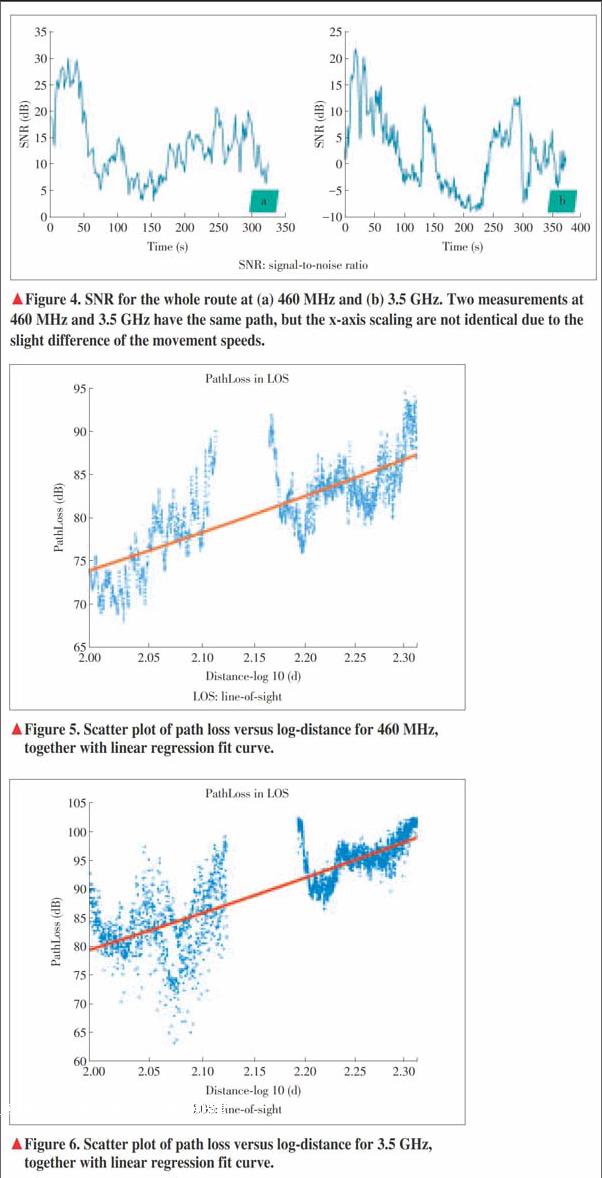
Fig. 3a shows the APDPs at 460 MHz， while Fig. 3b shows the APDPs at 3.5 GHz. We can see that there are clear LOS components and a few scattering components in most locations. Because we have the same velocity of trolley and route for the 460 MHz and 3.5 GHz measurements， both of the two APDPs have similar shapes and change trends. Fig. 4 shows the signal?to?noise ratio （SNR） calculated from the received signals through the whole route at 460 MHz （Fig. 4a） and 3.5 GHz （Fig. 4b）. It is obviously that the SNR at 460 MHz is larger than that at 3.5 GHz with nearly 10 dB. We excluded the measured data whose SNR is too low in order to get more accurate results for the analysis of channel parameters.

The two buildings in green circles in Fig. 2b are considered to be the reflectors which lead to the two multi?path components in Fig. 3a. The left building results in the multi?path component between 80 s to 170 s， and the right building leads to another multipath component （between 230 s to 300 s）. At the same time， the multi?path components are more blurred at 460 MHz. The reason is the difference of the free?space transfer loss between two frequency bands. The lower frequency band （460 MHz） has larger receive power and more scattering components. In addition， there are some weak power areas in the middle of graphics （between 170 s to 230 s）， they are mainly caused by the buildings and longer propagation distance in the measurement run.

3.2 Path Loss

where [γ] is the path loss exponent and PL（d0） is the intercept value of the path loss model at the reference distance d0 [12]. [Xδ]is a zero?mean Gaussian distributed random variable describing the random shadowing [13]. [γ]= 2 in free space. However， [γ] is generally higher for a realistic channel.

In this paper， we use the first path in PDP to determine the propagation distance between the transmitter and receiver. Here we should note the error of distance. The bandwidth is 30 MHz， resulting in a delay resolution of 33.33 ns corresponding to a distance 10 m. Because the true LOS path is located between two samples， there are less than 10?meter distance estimation error. Then， we transform the measured path loss from the time index to distance index.

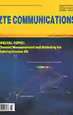
Fig. 5 describes the scatter plot of path loss versus log?distance for 460 MHz， together with linear regression fit curve， and Fig. 6 shows the corresponding results for 3.5 GHz.

Because the amount of measurement data in the NLOS scenario is less and the maximum and minimum distance difference is too small to obtain accurate linear regression results， we only consider the LOS scenario. Based on the measurements， the [γ] and PL（d0） are shown in Table 2. It is found that [γ]=4：23 and PL（d0）=-10：5 at 460 MHz， while [γ]=6：16 and PL（d0）=-43：5 at 3.5 GHz. According to [14]-[16]， [γ] should be between 2 to 5 in typical urban environments. A large value of [γ] at 3.5 GHz may be caused by the high frequency band and the difference between campus and urban.

3.3 Shadow Fading

According to [17]， after removing the distance?dependence from the received power， we obtain [Xδ]， which is the shadow fading component. Shadow fading in the dB scale can be modeled as a zero?mean Gaussian process with a standard deviation of σ [18]. Fig. 7 shows the probability density function （PDF） of the measured shadow fading components， together with the Gaussian distribution fit. We can found that σ =3.304 dB at 460 MHz and σ =4.208 dB at 3.5 GHz in the LOS scenario. It is noted that the model parameters above are limited by our measurement configurations.

3.4 Delay Spread

Root?mean?square （RMS） delay spread is the square root of the second central moment of a power?delay profile and is widely used to characterize the delay dispersion/frequency selectivity of the channel. It is the standard deviation about the mean excess delay [19] and defined as

[τrmsd=pAPDP（d，τp）τp2pAPDP（d，τp）-pAPDP（d，τp）τppAPDP（d，τp）2，] （7）

where τp represents the delay and APDP（d， τp） describes the corresponding delay power of the pth path measured at the location d. The RMS delay spread is a good measure of the multipath spread. It is also used to give an estimate of the maximum data rate for transmission.

Fig. 8 shows the cumulative distribution function （CDF） of the estimated RMS delay spread for both LOS and NLOS scenarios. We present RMS delay spread for two scenarios on one CDF curve， so that we can compare the differences between two frequency bands for the entire path comprehensively. It is found that there is a mean value of 84.5 ns at 460 MHz band and 35.5 ns at 3.5 GHz band. The measurement at 3.5 GHz has a lower delay spread than at 460 MHz， the reason is the low frequency band has a lower propagation loss and better propagation characteristics. Therefore， the lower frequency band has a higher SNR for the same measurement route， at the same time， can capture rich multi?path components. In the NLOS scenario， the measured RMS delay spread at some locations is larger than 200 ns， which is far higher than the LOS scenario. On the other hand， in the LOS scenario without obvious multi?path components， the measured RMS delay spread has its minimum value （about 20-40 ns）. Because of some obvious multipath components （highlighted in Fig. 3）， there is a larger measured RMS delay spread compared with， which is consistent with many previous measurements.

4 Conclusions

In this paper， measurements?based channel characterizations are presented for campus scenarios at 460 MHz and 3.5 GHz carrier frequencies， with a bandwidth of 30 MHz. Using the measured data， we analyze key channel parameters， such as power delay profile， path loss exponent， shadow fading， and delay spread. A path loss exponent is found to be 4.23 for 460 MHz and 6.16 for 3.5 GHz in the LOS scenario. RMS delay spread has a mean value of 84.5 ns for 460 MHz and 35.5 ns for 3.5 GHz. The results in this paper are helpful for 5G channel modeling， system simulation， and communication system design.

References

[1] R. He， Z. Zhong， B. Ai， et al.， “High?speed railway communications： from GSM?R to LTE?R，” IEEE Vehicular Technology Magazine， vol. 11， no. 3， pp. 49-58， 2016. doi： 10.1109/MVT.2016.2564446.

[2] M. J. Marcus， “5G and ‘IMT for 2020 and beyond [spectrum policy and regulatory issues]”， IEEE Wireless Communications， vol. 22， no. 4， pp. 2-3， 2015. doi： 10.1109/MWC.2015.7224717.

[3] ITU?R， “IMT vision—framework and overall objectives of the future development of IMT for 2020 and beyond，” Rec. ITU?R M. 2083， Feb. 2014.

[4] R. He， M. Yang， L. Xiong， et al.， “Channel measurements and modeling for 5G communication systems at 3.5 GHz band，” in URSI Asia?Pacific Radio Science Conference， Seoul， South Korea， Aug. 2016， pp. 1855-1858. doi： 10.1109/URSIAP?RASC.2016.7601208.

[5] R. He， A. F. Molisch， F. Tufvesson， et al.， “Vehicle?to?vehicle propagation models with large vehicle obstructions，” IEEE Transactions on Intelligent Transportation Systems， vol. 15， no. 5， pp. 2237-2248， 2014. doi： 10.1109/TITS.2014.2311514.

[6] T. K. Sarkar， Z. Ji， K. Kim， et al.， “A survey of various propagation models for mobile communication，” IEEE Antennas and Propagation Magazine， vol. 45， no. 3， pp. 51-82， 2003. doi： 10.1109/MAP.2003.1232163.

[7] T. S. Rappaport， S. Y. Seidel， and K. Takamizawa， “Statistical channel impulse response models for factory and open plan building radio communicate system design，” IEEE Transactions on Communications， vol. 39， no. 5， pp. 794-807， 1991. doi： 10.1109/26.87142.

[8] R. He， W. Chen， B. Ai， et al.， “On the clustering of radio channel impulse responses using sparsity?based methods，” IEEE Transactions on Antennas and Propagation， vol. 64， no. 6， pp. 2465-2474， 2016. doi： 10.1109/TAP.2016. 2546953.

[9] H. L. Bertoni， Radio Propagation for Modern Wireless Systems. London， UK： Pearson Education， 1999.

[10] J. B. Andersen， T. S. Rappaport， and S. Yoshida， “Propagation measurements and models for wireless communications channels，” IEEE Communications Magazine， vol. 33， no. 1， pp. 42-49， 1995. doi： 10.1109/35.339880.

[11] X. Yin and X. Cheng. Propagation Channel Characterization， Parameter Estimation， and Modeling for Wireless Communications. Hoboken， USA： John Wiley & Sons， 2016.

[12] R. He， Z. Zhong， B. Ai， et al.， “An empirical path loss model and fading analysis for high?speed railway viaduct scenarios，” IEEE Antennas and Wireless Propagation Letters， vol. 10， pp. 808-812， 2011. doi： 10.1109/LAWP.2011. 2164389.

[13] R. He， Z. Zhong， B. Ai， and J. Ding， “Propagation measurements and analysis for high?speed railway cutting scenario，” Electronics Letters， vol. 47， no. 21， pp. 1167-1168， 2011. doi： 10.1049/el.2011.2383.

[14] V. S. Abhayawardhana， I. J. Wassell， D. Crosby， M. P. Sellars， and M. G. Brown， “Comparison of empirical propagation path loss models for fixed wireless access systems，” in IEEE 61st Vehicular Technology Conference， VTC 2005?Spring， Stockholm， Sweden. doi： 10.1109/VETECS.2005.1543252.

[15] ITU? R， “Guidelines for evaluation of radio interface technologies for IMT?Advanced，” Rep. ITU?R M. 2135， 2008.

[16] S. Rangan， T. S. Rappaport， and E. Erkip， “Millimeter?wave cellular wireless networks： potentials and challenges，” Proceedings of the IEEE， vol. 102， no. 3， pp. 366-385， Mar. 2014. doi： 10.1109/JPROC.2014.2299397.

[17] A. F. Molisch， Wireless Communications， 2nd ed. Hoboken， USA： Wiley， 2010.

[18] R. He， Z. Zhong， B. Ai， et al. “Measurements and analysis of propagation channels in high?speed railway viaducts，” IEEE Transactions on Wireless Communications， vol. 12， no. 2， pp. 794-805， 2013. doi： 10.1109/TWC.2012.120412. 120268.

[19] P. Bello， “Characterization of randomly time?variant linear channels，” IEEE Transactions on Communications Systems， vol. 11， no. 4， pp. 360-393， 1963. doi： 10.1109/TCOM.1963.1088793.

Manuscript received： 2017?2?12