P.MOKHTARY

Department of Mathematics，Faculty of Basic Sciences，Sahand University of Technology，Tabriz，Iran

E-mail∶mokhtary.payam@gmail.com；mokhtary@sut.ac.ir



DISCRETE GALERKIN METHOD FOR FRACTIONAL INTEGRO-DIFFERENTIAL EQUATIONS∗

P.MOKHTARY

Department of Mathematics，Faculty of Basic Sciences，Sahand University of Technology，Tabriz，Iran

E-mail∶mokhtary.payam@gmail.com；mokhtary@sut.ac.ir

In this article，we develop a fully Discrete Galerkin（DG）method for solving initial value fractional integro-differential equations（FIDEs）.We consider Generalized Jacobi polynomials（GJPs）with indexes corresponding to the number of homogeneous initial conditions as natural basis functions for the approximate solution.The fractional derivatives are used in the Caputo sense.The numerical solvability of algebraic system obtained from implementation of proposed method for a special case of FIDEs is investigated.We also provide a suitable convergence analysis to approximate solutions under a more general regularity assumption on the exact solution.Numerical results are presented to demonstrate the effectiveness of the proposed method.

Fractional integro-differential equation（FIDE）；Discrete Galerkin（DG）；Generalized Jacobi Polynomials（GJPs）；Caputo derivative

2010 MR Subject Classification34A08；65L60

1　Introduction

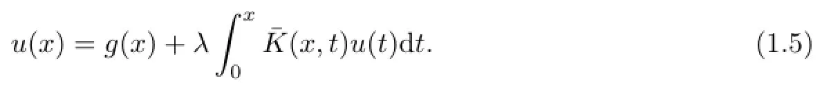
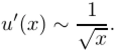
In this article，we provide a convergent numerical scheme for solving FIDE

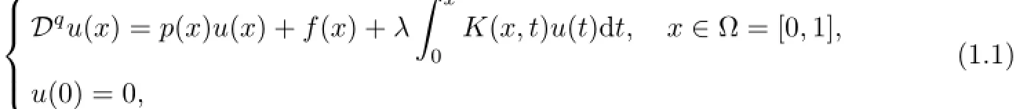
where q∈R+∩（0，1）.The symbol R+is the collection of all positive real numbers.p（x）and f（x）are given continuous functions and K（x，t）is a given sufficiently smooth kernel function，and u（x）is the unknown function.

Noting that the condition u（0）=0 is not restrictive，due to the fact that（1.1）with nonhomogeneous initial condition u（0）=d，d 6=0 can be converted to the following homogeneous FIDE

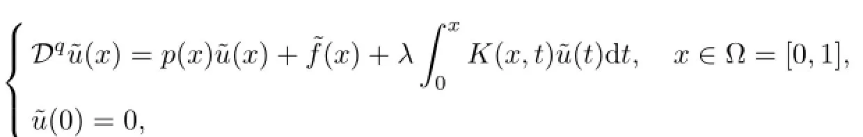
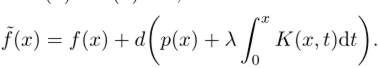
by the simple transformation˜u（x）=u（x）−d，where

Such kind of equations arise in the mathematical modeling of various physical phenomena，such as heat conduction，materials with memory，combined conduction，convection and radiation problems（［3，5，29，30］）.

Dqu（x）denotes the fractional Caputo differential operator of order q and is defined as（［8，19，31］）

where

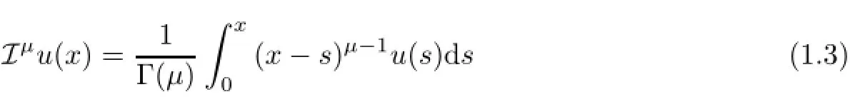
is the fractional integral operator from orderµ.Γ（µ）is the well known Gamma function.The following relation holds［8］

From the relation above，it is easy to check that（1.1）is equivalent to the following weakly singular Volterra integral equation

·f（x）∈Cl（Ω），l≥1，

·p（x）∈Cl（Ω），l≥1，

·K（x，t）∈Cl（D），D=｛（x，t）；0≤t≤x≤1｝，l≥1，

·K（x，x）6=0，

then the regularity of the unique solution u（x）of（1.5）and also（1.1）is described by

where the coefficients γj，kare s∪ome constants，Ul（.；q）∈Cl（Ω），and（j，k）：=｛（j，k）：j，k∈N0，j+kq＜l｝.Here，N0=N｛0｝，where the symbol N denotes the collection of all natural numbers.Thus，we must expect the first derivative of the solution to has a discontinuity at the origin.More precisely，if the given functions g（x），p（x），and K（x，t）are real analytic in their domains，then it can be concluded that there is a function U=U（z1，z2）that is real and analytic at（0，0），so that solutions of（1.5）and also（1.1）can be written as u（x）=U（x，xq）（［4，35］）.

Recently，several numerical methods for the numerical solution of FIDE's were proposed；see［2，11，12，15，20-28，33，36，38，39］.In［2］，an analytical solution for a class of FIDE's was proposed.In［11］，authors applied collocation method to solve the nonlinear FIDE's.In［15］，Taylor expansion approach was presented for solving a class of linear FIDE's including those of Fredholm and Volterra types.In［20］，Chebyshev pseudospectral method was implemented to solve linear and nonlinear system of FIDE's.Adomian decomposition method to solve nonlinear FIDE's was proposed in［21］.In［22］，authors solved FIDE's by adopting hybrid collocation method to an equivalent integral equation of convolution type.In［23］，authors proposed an analyzed spectral Jacobi collocation method for the numerical solution of general linear FIDE's.In［24］，Mokhtary and Ghoreishi proved the L2convergence of Legendre Tau method for the numerical solution of nonlinear FIDE's.In［28］，fractional differential transform method was developed to solve FIDE's with nonlocal boundary conditions.In［33］，Rawashdeh studied the numerical solution of FIDE's by polynomial spline functions.In［36］，authors solved fractional nonlinear Volterra integro differential equations using the second kind Chebyshev wavelets.

Many of the techniques mentioned above or have not proper convergence analysis or if any，very restrictive conditions including smoothness of the exact solution are assumed.In this article we will consider non-smooth solutions of（1.1）.In this case，although the DG method can be implemented directly，but this method leads to a very poor numerical results. Thus，it is necessary to introduce a regularization procedure that allows us to improve the smoothness of the given functions and then to approximate the solution with a satisfactory order of convergence.To this end，we introduce a simple variable transformation for the regularization of solutions of the original equation such that the resulting equation possesses a more regularity properties.The main advantage of our proposed method is that in spite of the singularity behavior of the exact solution，it possesses a high order accuracy under a more general regularity assumptions on the exact solution and input data.Our logic in choosing proper transformation is based on the formal asymptotic expansion of the exact solution in（1.6）.Considering（1.1）and using the variable transformation

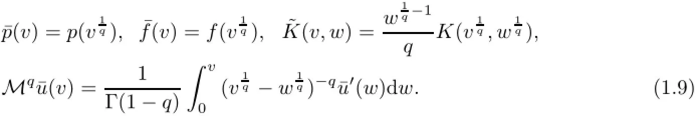
we can change（1.1）to the following equation

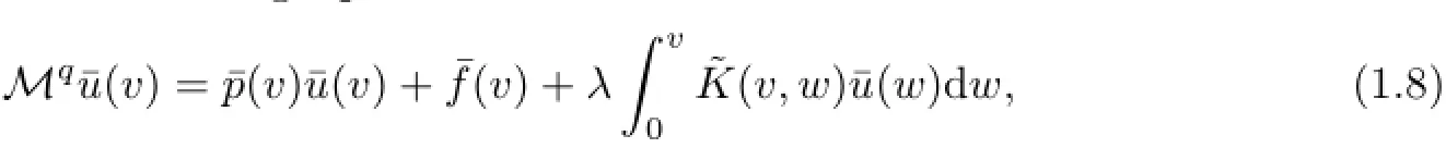
where

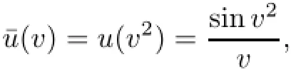
From（1.6），the exact solution¯u（v）can be written asIt can be seen that¯u′（v）∈C（Ω）.It is trivial that forthe unknown

function¯u（v）will be in the form

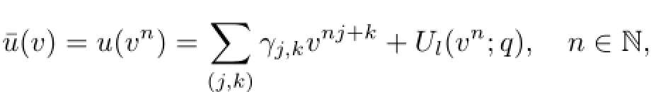
which is infinitely smooth.Then，we can deduce that the solution¯u（v）of the new equation（1.8）possesses a better regularity and DG theory can be applied conveniently to obtain a high order accuracy.

In the sequel，we introduce the DG solution¯uN（v）based on GJPs to（1.8）.As the exact solutions of（1.1）can be written as u（x）=¯u（v），then we define uN（x）=¯uN（v），x，v∈Ω as the approximate solution of（1.1）.

Spectral Galerkin method is one of the weighted residual methods（WRM），in which approximations are defined in terms of truncated series expansions，such that residual，which should be exactly equal to zero，is forced to be zero only in an approximate sense.It is well knownthat，in this method，the expansion functions must satisfy in the supplementary conditions. The two main characteristics behind the approach are that first it reduces the given problems to those of solving a system of algebraic equations，and in general converges exponentially and almost always supplies the most terse representation of a smooth solution（［6，16，34］）.

In this article，we use shifted GJPs on Ω，which are mutually orthogonal with respect to the shifted weight function δα，β（v）=（2−2v）α（2v）βon Ω，where α，β belong to one of the following index sets：

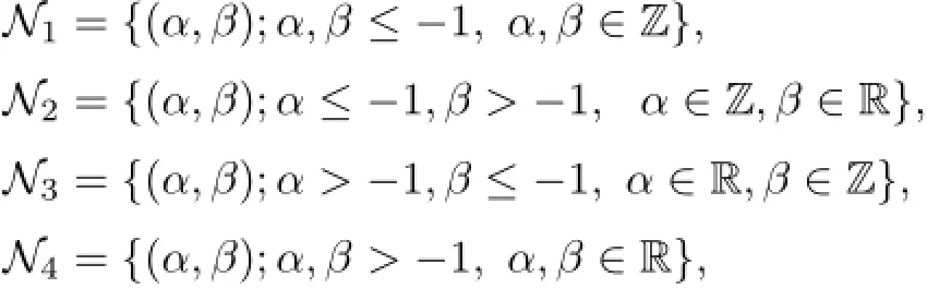
where the symbol Z is the collection of all integer numbers.The main advantage of GJPs is that these polynomials，with indexes corresponding to the number of homogeneous initial conditions in a given FIDE，are the natural basis functions to the Galerkin approximation of this problem（［13，14］）.

The organization of this article is as follows：We begin by reviewing some preliminaries，which are required for establishing our results in Section 2；In Section 3，we introduce the DG method based on the GJPs and its application to（1.8）；Numerical solvability of the algebraic system obtained from DG discretization of a special case of（1.8）with 0＜q＜12and¯p（v）=1 based on GJPs is given in Section 4；Convergence analysis of the proposed scheme is provided in Section 5；Numerical experiments are carried out in Section 6.

2　Preliminaries and Notations

In this section，we review the basic definitions and properties that are required in the sequel.

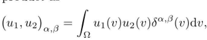
Defining weighted inner product as

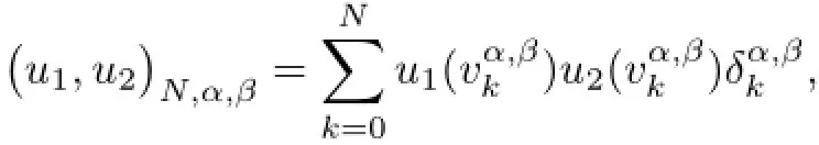
and discrete Jacobi-Gauss inner product as

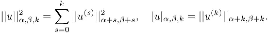
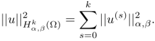
we recall the following norms over Ω

The non-uniformly Jacobi-weighted Sobolev space is denoted by（Ω）and is defined as

equipped with the norm and semi-norm

equipped with the norm

We denote the shifted GJPs on Ω by（v）and define it as

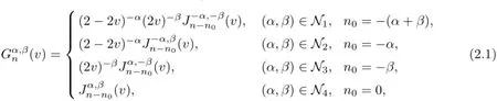
From（2.1）and the following formula［9］

we can obtain the following explicit formula for（v），

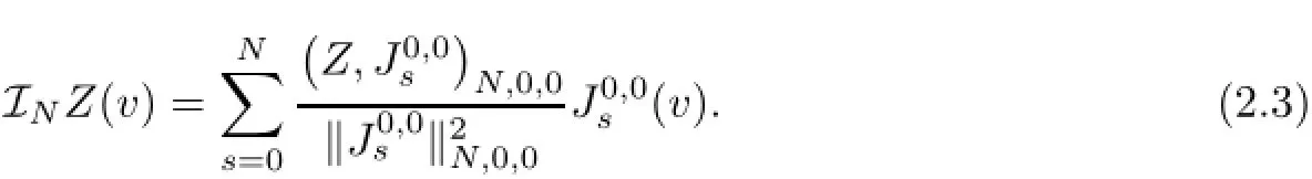
For any continuous function Z（v）on Ω，we define the Legendre Gauss interpolation operator INas

Let PNbe the space of all algebraic polynomials of degree up to N.We introduce the Legendre projection ΠN：L2（Ω）→PNwhich is a mapping such that for any Z（v）∈L2（Ω），

3　DG Approach

In this section，we present the numerical solution of（1.8）using the DG method based on GJPs.

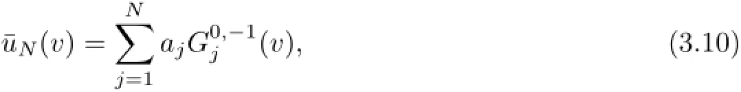
Let

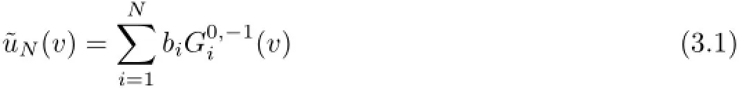
be the Galerkin solution of（1.8）.It is trivial that˜uN（0）=0.

Galerkin formulation of（1.8）is to find˜uN（v），such that

Applying transformation w（θ）=vθ，for θ∈Ω，we obtain

Substituting（3.3）in（3.2）yields

Inserting（3.1）in（3.4），we get

Now，we try to find an explicit form forTo this end，using（2.2）we have

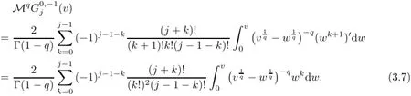
Applying relation［12］，

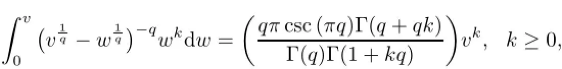
in（3.7）we can obtain the following explicit formula for

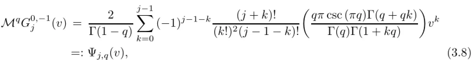
Substituting（3.8）in（3.6），we obtain

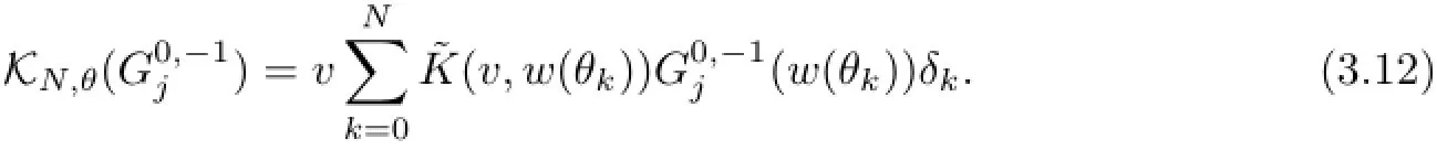
In this position，we approximate the integral terms of（3.9）using（N+1）−point Legendre Gauss quadrature formula.Our DG method is to seek

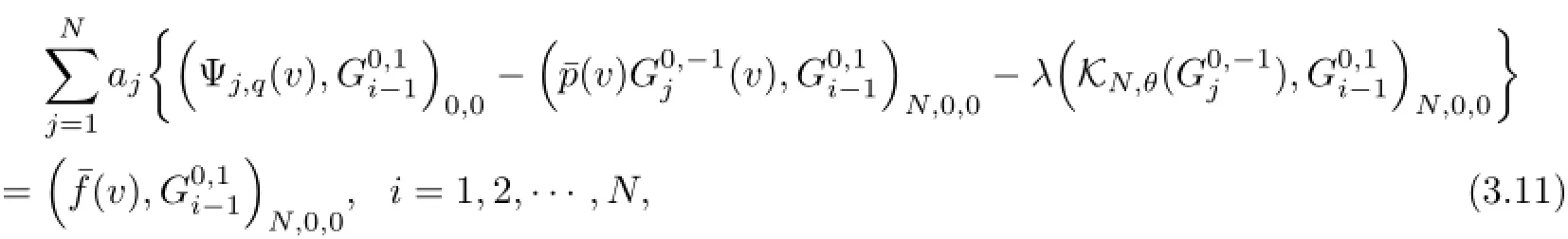
where

It is trivial that the solution of（3.11）gives us unknown coefficientsin（3.10）.

4　Existence and Uniqueness Theorem for DG Algebraic System

The main object of this section is to provide an existence and uniqueness Theorem for a special case of the DG algebraic system of equations（3.11）with¯p（v）=1 and 0＜q＜12. Throughout this article，Ciwill denote a generic positive constant that is independent on N.

First，we give some preliminaries，which will be used in the sequel.

Definition 4.1Let X，Y be normed spaces.A linear operator A：X→Y is compact if the set｛Ax|||x||X≤1｝has compact closure in Y.

Theorem 4.2（［17，18，37］）Assume that X and Y be two Banach spaces.Let

be a linear operator equation，where A：X→Y is a linear continuous operator，and the operator I−A is continuously invertible.As an approximation solution of（4.1），we consider the equation

which can be rewritten as

where ANis a linear continuous operator in a closed subspace˜Y of Y.BN，˜BN：Y→˜Y are linear continuous projection operators and SN=AN−˜BNA is a linear operator in˜Y.If the following conditions are fulfilled：

·For any Z∈˜Y，we have‖SNZ‖→0 as N→∞，

·‖A−˜BNA‖→0 as N→∞，

·‖f−BNf‖→0 as N→∞，

then（4.3）possesses a unique solution vN∈˜Y for a sufficiently large N.

Lemma 4.3（［1］）Let X and Y be Banach spaces and˜Y be a subspace of Y.Let˜BN：Y→˜Y be a family of linear continuous projection operators with

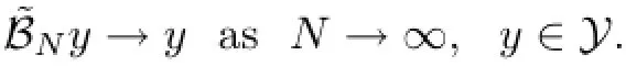
Assume that linear operator A：X→Y is compact.Then，

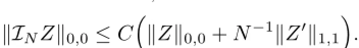
Lemma 4.4（［34］）（Interpolation error bound）Let INZ be the interpolation polynomial approximation of the function Z（v）defined in（2.3）.For any Z（v）∈（Ω）with k≥1，we have

Lemma 4.5（［7］）For every bounded function Z（v），there exists a constant C independent of Z such that

Lemma 4.6（［34］）（Legendre Gauss quadrature error bound）If Z（v）∈（Ω）for some k≥1 and Φ∈PN，then for the Legendre Gauss integration，we have

Now，we intend to prove the existence and uniqueness Theorem for a special case of the DG system（3.11）with¯p（v）=1 and 0＜q＜

Theorem 4.7（Existence and Uniqueness）Let 0＜q＜，¯p（v）=1，and¯f（v）∈（Ω）with k≥1.If（1.8）has a uniquely solution¯u（v），then the linear DG system（3.11）has a unique solution¯uN（v）∈PNfor sufficiently large N.

ProofOur strategy in Proof is based on two steps.First，we try to represent（3.11）in the operator form（4.3）and afterwards we apply Theorem 4.2 to this operator form to conclude the desired result.

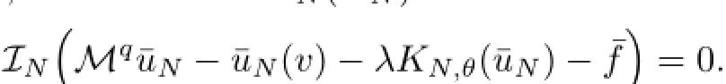
Step 1In this step，we show that the DG system（3.11）can be written in the operator form（4.3）.To this end，consider（1.8）and define

According to the proposed method，we have

From interpolation and Legendre Gauss quadrature properties，we can write

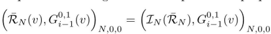
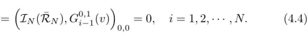
Using（4.4）and（4.5），we can deduce）=0 and so

The equation above can be rewritten as

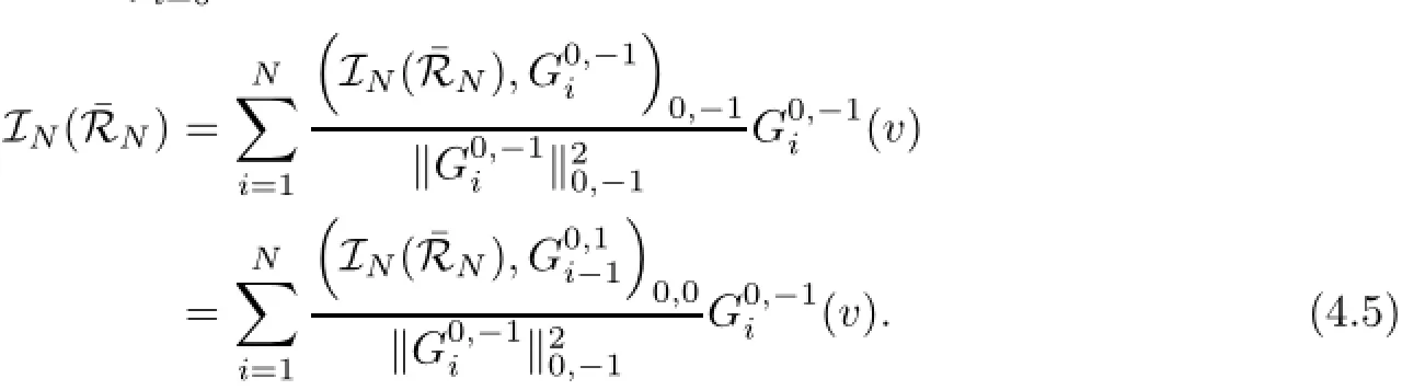
and thereby

where INand ΠNare defined in（2.3）and（2.4）respectively and

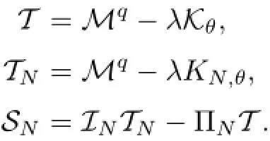
As（4.7）is the form in which the DG method is implemented，it leads directly to the equivalent linear system（3.11）.Thus，the existence and uniqueness of solutions of（4.7）approve the existence and uniqueness of solutions of（3.11）.In this position，we can write（4.7）in operator form（4.3）by considering so it is the desired result of this step.

Step 2In this step，we intend to apply Theorem 4.2 with the assumptions（4.8）to prove the Theorem.To this end，following Theorem 4.2 we must show that

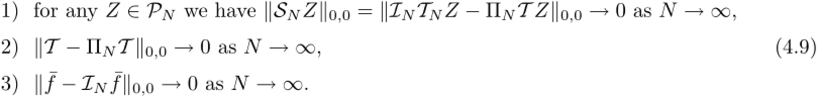
First，we prove the first condition in（4.9）.For this，we can write

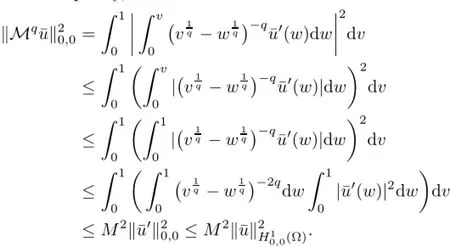
Since we have MqZ∈PNfor any Z∈PN，then

Using Lemmas 4.5 and 4.6 and relations（3.3）and（3.12），we can obtain

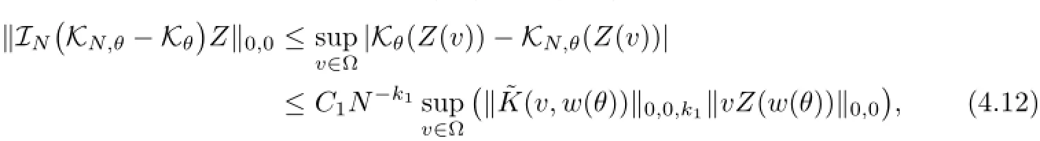
Substituting（4.12）and（4.14）in（4.11），we can conclude the first condition in（4.9）.Applying Lemma 4.4 gives us the third condition in（4.9）.To complete the proof，it is sufficient that we prove the second condition of（4.9）.To this end，we apply Lemma 4.3 with the assumptions（4.8）.Becausethe second condition in（4.9）can be achieved by showing compactness of the operator T.a continuous kernel，then the operator T will be compact ifcompact operator.For this，defineusing Cauchy-Schwartz inequality，we have

In this position，all conditions in（4.9）that are required to deduce the existence and uniqueness of solutions of the DG system（3.11）are proved and then the proof is completed.

5　Convergence Analysis

In this section，we will try to provide a reliable convergence analysis，which theoretically justify the convergence of the proposed approximate method for the numerical solution of（1.1）with p（x）=1.

In the sequel，our discussion is based on these lemmas：

Lemma 5.1（［34］）For any Z（x）∈（Ω），we have

Lemma 5.2（［19］，Lemma 2.1（a））The fractional integral operator Iµis bounded in L2（Ω）and

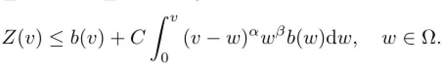
Lemma 5.3（［7］）（Gronwall inequality）Assume that Z（v）is a non-negative，locally integrable function defined on Ω satisfing

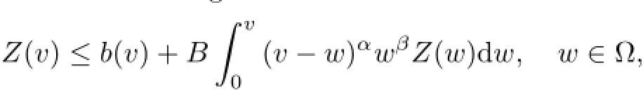
where α，β＞−1，b（v）≥0 and B≥0.Then，there exists a constant C such that

Now，we state and prove the main result of this section regarding the error analysis of the proposed method for the numerical solution of（1.1）with p（x）=1.

Theorem 5.4（Convergence）Let u（x）and¯u（v）be the exact solutions of equations（1.1）and（1.8），respectively，that are related by u（x）=¯u（v）.Assume that uN（x）=¯uN（v）is the approximate solution of（1.1），where¯uN（v）is DG solution of the transformed equation（1.8）. If the following conditions are fulfilled：

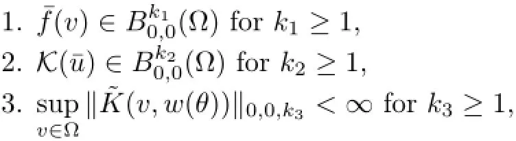
then for sufficiently large N，we have

ProofAs we point out in the previous section，DG solution¯u（v）satisfied in the regularized equation（4.6）.As Mq¯uNis a polynomial from degree of at most N，then we can rewrite（4.6）as

Subtracting（1.8）from（5.1）and some simple manipulations，we obtain

Applying transformation（1.7）to the operator Iqu，we get

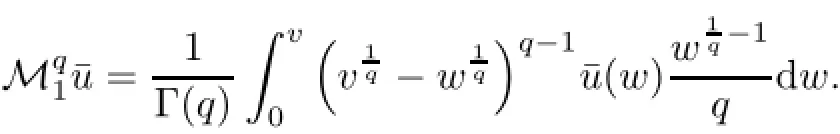
Following（1.4），it is easy to check that

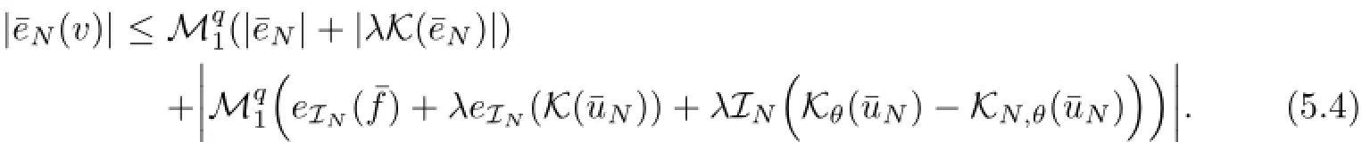
Since

then（5.4）can be rewritten as

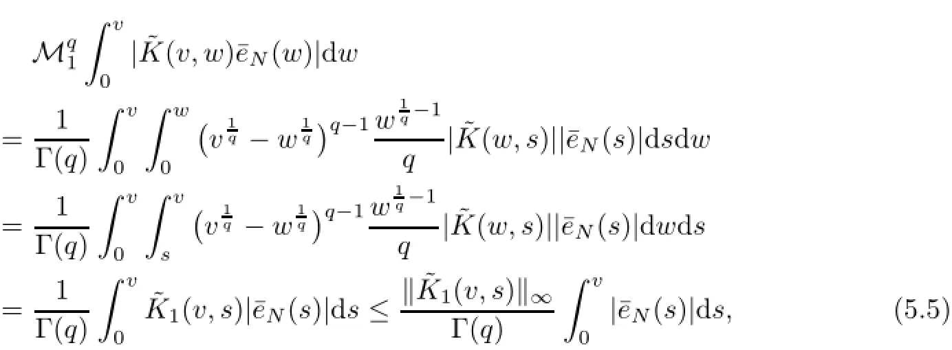
where

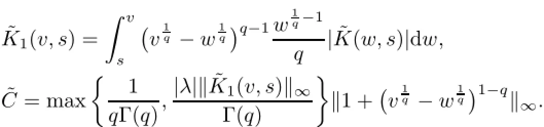
Using Gronwall inequality（Lemma 5.3）in（5.6）yields

It can be checked that by applying transformation（1.6），we get

where Z（x）is a given function and¯Z（v）=Z（v1q）.Using relations（5.8）and（5.9）in（5.7），we have

In contrast，by applying（1.6）and Lemma 5.2，we can obtain

where

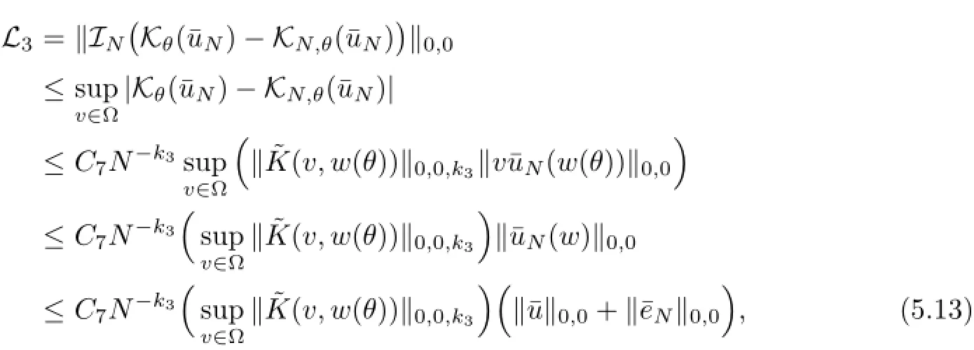
Now，it is sufficient to find suitable upper bounds to the above norms.According to Lemma 4.4，we have

Using Lemmas 4.5 and 4.6，we can obtain

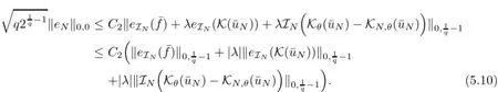
For sufficiently large N，the desired result can be concluded by inserting（5.12）and（5.13）in（5.11）.

6　Numerical Results

In this section，we apply a program written in Mathematica to some numerical examples to demonstrate the accuracy of the proposed method and effectiveness of applying regularization process.the”Numerical Error”always refers to the L2-norm of the obtained error function.

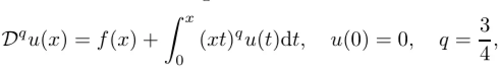
Example 6.1Consider the following FIDE，

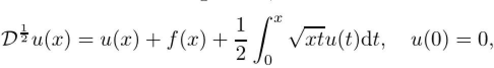
with the exact solution u（x）=and

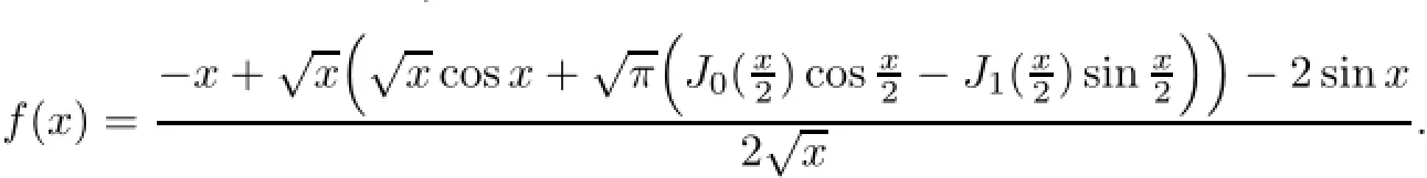
Here，Jn（z）gives the Bessel function of the first kind.

This example has a singularity at the origin，that is，

In the theory presented in the previous section，our main concern is the regularity of the transformed solution.For this problem，by applying coordinate transformation x=v2，t=w2，

the infinitely smooth solution，

is obtained.The main purpose is to check the convergence behavior of the numerical solutions with respect to the approximation degree N.Numerical results obtained are given in Table 1 and Figure 1.As expected，the errors show an exponential-like decay，because in this semi-log representation（Figure 1）one observes that the error variations are essentially linear versus the degrees of approximation.

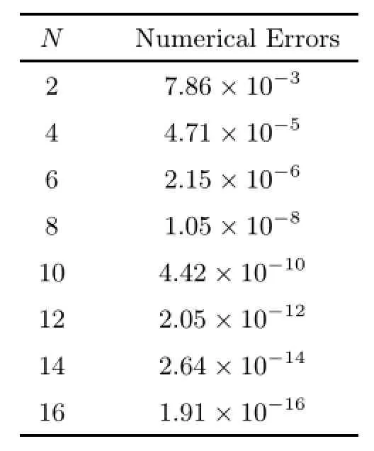
Table 1The numerical errors of Example 6.1

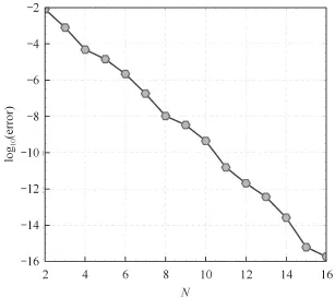
Figure 1The numerical errors of Example 6.1 with various values of N

Example 6.2（［24］）Consider the following FIDE

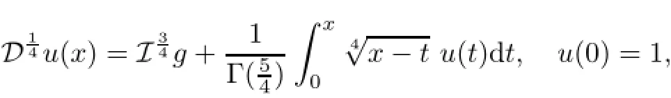
As this example has nonhomogeneous initial condition，first，we convert it to the following homogeneous FIDE

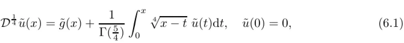
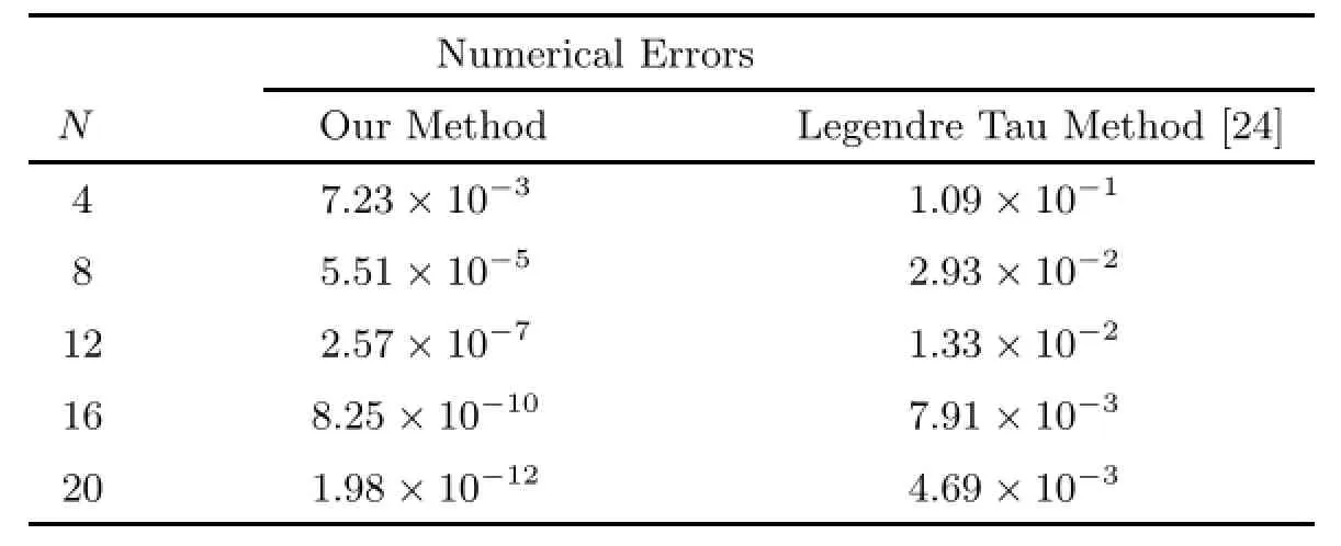
Table 2The numerical errors of Example 6.2

Figure 2Obtained errors versus N，when Legendre Tau and proposed DG methods are used to obtain an approximate solution for Example 6.2

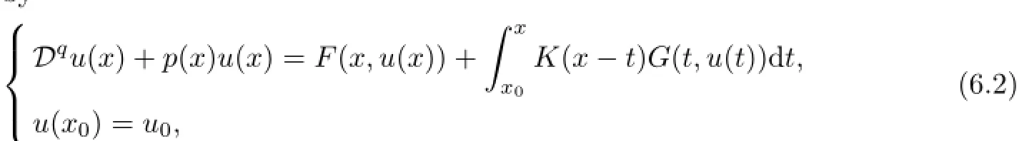
Example 6.3（［10］）Some physical phenomena involving certain type of memory effects are represented byin Banach space X，where 0＜q≤1.Functions p（x）and K（x，t）are a continuous function and a real valued locally integrable function on Ω，respectively.Nonlinear maps F and G are defined on Ω×X into X.

Here，we consider（6.2）with following assumptions：

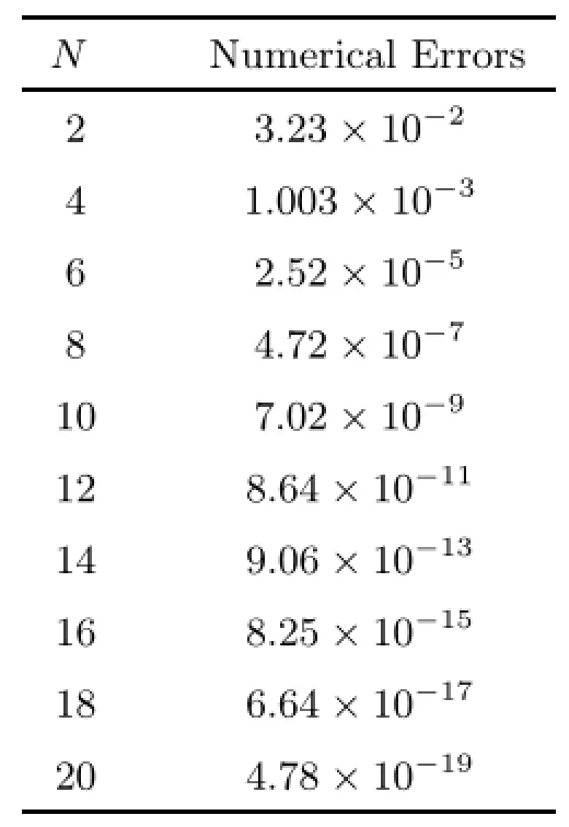
Table 3The numerical errors of Example 6.3

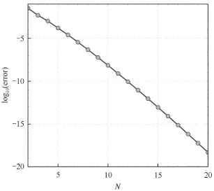
Figure 3The numerical errors of example 6.3 with various values of N

where BesselI［n，z］gives the modified Bessel function of the first kind Jn（z）.Following assumptions（6.3），the exact solution of（6.2）is given by u（x）=ex√x.Now，we solve this problem by the proposed numerical method in Section 3.Obtained numerical results are given in Table 3 and Figure 3.Our results show that the proposed regularization process works well and regardless of the singularity behavior of the exact solution，the approximate results are in a goodagreement with the exact one.Indeed，we observe from Figure 3 that the obtained approximation errors decay exponential-like versus the approximation degree N，because in semi-log representation one observes that error variations are linear versus N.It is easy to check that these results approve the obtained theoretical prediction in Theorem 5.4（ξ=∞）.

Example 6.4Consider the following FIDE

with the exact solution u（x）=x−qlog（x+1）and

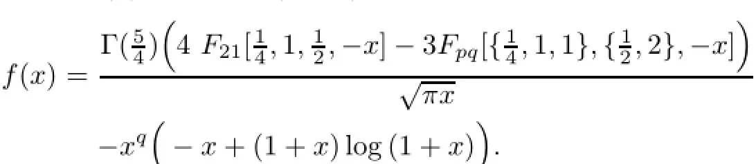
Here，F21［a；b；c；z］and Fpq［a；b；z］are the well known Hypergeometric and Generalized Hypergeometric functions，respectively.

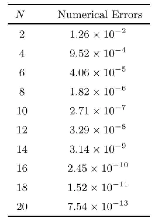
Table 4The numerical errors of Example 6.4

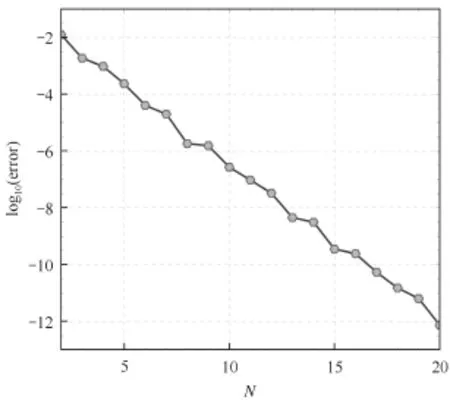
Figure 4The numerical errors of Example 6.4 with various values of N

The numerical results obtained are given in Table 4 and Figure 4.Clearly，the proposed approximate scheme is powerful and the obtained results are in a good agreement with the exact ones.

References

［1］Atkinson K E.The Numerical Solution of Integral Equations of the Second Kind.Cambridge，1997

［2］Awawdeh F，Rawashdeh E A，Jaradat H M.Analytic solution of fractional integro-differential equations. Ann Univ Craiova Math Comput Sci Ser，2011，38：1-10

［3］Bagley R L，Torvik P J.A theoretical basis for the application of fractional calculus to viscoelasticity.J Rheol，1983，27：201-210

［4］Brunner H.Collocation Methods for Volterra and Related Functional Equations.Cambridge：Cambridge University Press，2004

［5］Caputo M.Linear models of dissipation whose Q is almost frequency independent II.Geophys J Roy Astron Soc，1967，13：529-539

［6］Canuto C，Hussaini M Y，Quarteroni A，Zang T A.Spectral Methods，Fundamentals in Single Domains. Berlin：Springer-Verlag，2006

［7］Chen Y，Tang T.Convergence analysis of the Jacobi spectral collocation methods for volterra integral equations with a weakly singular kernel.Math Comput，2010，79：147-167

［8］Diethelm K.The Analysis of Fractional Differential Equations.Berlin：Springer-Verlag，2010

［9］Doha E H，Bhrawy A H，Ezz-Eldien S S.A new Jacobi operational matrix：an application for solving fractional differential equations.Appl Math Model，2012，36：4931-4943

［10］El-Borai Mahmoud M，Debbouche Amar.On some fractional integro-differential equations with analytic semigroups.Int J Contemp Math Sciences，2009，4（28）：1361-1371

［11］Eslahchi M R，Dehghan M，Parvizi M.Application of the collocation method for solving nonlinear fractional integro-differential equations.J Comput Appl Math，2014，257：105-128

［12］Ghoreishi F，Mokhtary P.Spectral collocation method for multi-order fractional differential equations.Int J Comput Math，2014，11（5）：23

［13］Guo Ben-Yu，Shen Jie，Wang Li-Lian.Optimal spectral-galerkin methods using generalized Jacobi polynomials.J Sci Comput，2006，27：305-322

［14］Guo Ben-Yu，Shen Jie，Wang Li-Lian.Generalized Jacobi polynomials/functions and their applications. Appl Numer Math，2009，59：1011-1028

［15］Huang L，Li X F，Zhao Y L，Duan X Y.Approximate solution of fractional integro-differential eqations by Taylor expansion method.Comput Math Appl，2011，62：1127-1134

［16］Hesthaven J S，Gottlieb S，Gottlieb D.Spectral Methods for Time-Dependent Problems.Cambridge University Press，2007

［17］Kantrovich L V.Functional analysis and applied mathematics.Usp Mat Nauk，1984，3：89-185

［18］Kantrovich L V，Akilov G P.Functional Analysis in Normed Spaces（Funktsional’nyi analiz v normirovannykh prostranstvakh）.Moscow：Fizmatgiz，1959

［19］Kilbas A A，Srivastava H M，Trujillo J J.Theory and Applications of Fractional Differential Equations. Amesterdam：Elsevier，2006

［20］Khader M M，Sweilam N H.On the approximate solutions for system of fractional integro-differential equations using chebyshev pseudo-spectral method.Appl Math Model，2013，27（24）：819-9828

［21］Mittal R C，Nigam R.Solution of fractional calculus and fractional integro-differential equations by adomian decomposition method.Int J Appli Math Mech，2008，4（4）：87-94

［22］Ma Xiaohua，Huang C.Numerical solution of fractional integro-differential equations by Hybrid collocation method.Appl Math Comput，2013，219：6750-6760

［23］Ma Xiaohua，Huang C.Spectral collocation method for linear fractional integro-differential equations.Appl Math Model，2014，38（4）：1434-1448

［24］Mokhtary P，Ghoreishi F.The L2-convergence of the Legendre spectral Tau matrix formulation for nonlinear fractional integro differential equations.Numer Algorithms，2011，58：475-496

［25］Mokhtary P，Ghoreishi F.Convergence analysis of spectral Tau method for fractional Riccati differential equations.Bull Iranian Math Soc，2014，40（5）：1275-1290

［26］Mokhtary P.Operational Tau method for non-linear FDEs.Iranian Journal of Numerical Analysis and Optimization，2014，4（2）：43-55

［27］Mokhtary P.Reconstruction of exponentially rate of convergence to Legendre-collocation solution of a class of fractional integro-differential equations.J Comput Appl Math，2014，279：145-158

［28］Nazari D，Shahmorad S.Application of the fractionl differential transform method to fractional-order integro-differential equations with nonlocal boundary conditions.J Comput Appl Math，2010，234：883-891

［29］Oldham K B，Spanier J.The Fractional Calculus.New York：Academic Press，1974

［30］Olmstead W E，Handelsman R A.Diffusion in a semi-infinite region with nonlinear surface dissipation. SIAM Rev，1976，18：275-291

［31］Podlubny I.Fractional Differential Equations.Academic Press，1999

［32］Porter D，Stirling David S G.Integral Equations，A Practical Treatment，from Spectral Theory to Applications.New York：Cambridge University Press，1990

［33］Rawashdeh E A.Numerical solution of fractional integro-differential equations by collocation method.Appl Math Comput，2006，176：1-6

［34］Shen Jie，Tang Tao，Wang Li-Lian.Spectral Methods，Algorithms，Analysis and Applications.Springer，2011

［35］Xianjuan Li，Tang T.Convergence analysis of Jacobi spectral collocation methods for Abel-Volterra integral equations of second kind.Front Math China，2012，7（1）：69-84

［36］Zhu Li，Fan Qibin.Numerical solution of nonlinear fractional order Volterra integro differential equations by SCW.Commun Nonlinear Sci Numer Simul，2013，18（15）：1203-1213

［37］Vainikko G M.Galerkin’s perturbation method and the general theory of approximate methods for nonlinear equations.USSR Computational Mathematics and Mathematical Physics，1967，7（4）：1-41

［38］Yang Yin.Jacobi spectral galerkin methods for fractional integro-differential equations.Calcolo.DOI：10.1007/s10092-014-0128-6.

［39］Yang Yin，Chen Yanping，Huang Yanqing.Convergence analysis of the Jacobi spectral-collocation method for fractional integro-differential equations.Acta Mathematica Scientia，2014，34B（3）：673-690

December 29，2014；revised May 15，2015.