Wenqiang ZHAO（赵文强）

School of Mathematics and Statistics，Chongqing Technology and Business University，Chongqing 400067，China

E-mail∶gshzhao@sina.com



REGULARITY OF RANDOM ATTRACTORS FOR A STOCHASTIC DEGENERATE PARABOLIC EQUATIONS DRIVEN BY MULTIPLICATIVE NOISE∗

Wenqiang ZHAO（赵文强）

School of Mathematics and Statistics，Chongqing Technology and Business University，Chongqing 400067，China

E-mail∶gshzhao@sina.com

We study the regularity of random attractors for a class of degenerate parabolic equations with leading term div（σ（x）∇u）and multiplicative noises.Under some mild conditions on the diffusion variable σ（x）and without any restriction on the upper growth p of nonlinearity，except that p＞2，we show the existences of random attractor in（DN，σ）∩L（DN）（∈［2，2p−2］）space，where DNis an arbitrary（bounded or unbounded）domain in RN，N≥2.For this purpose，some abstract results based on the omega-limit compactness are established.

Random dynamical systems；stochastic degenerate parabolic equation；multiplicative noise；random attractors；Wiener process 2010 MR Subject Classification35B40；35B41；60H15

1　Introduction

In this article，we study the regularity of random attractors for the following stochastic degenerate parabolic equation

on an arbitrary（bounded or unbounded）domain DN⊆RN，N≥2，with the initial value and boundary conditions

where t＞τ，x∈DN，∂DNis the boundary of DN，W（t）=（W1（t），W2（t），···，Wm（t））is a mutually independent two-sided real-valued Wiener process defined on the m-dimensional canonical Wiener probability space（Ω，F，P），which will be specified later.

In the deterministic case（that is，bj=0，j=1，2，···，m），the problems with diffusion variable model several physical phenomena，where the spatial heterogeneity has an importantrole，such as the heat propagation in heterogeneous materials［1］，the transport of electron temperature in a confined plasm［2］，the evolution problems of a biological population［3］，and the growth and control of brain tumors［4］.

In this article，we assume that the diffusion variable σ：DN→［0，+∞）satisfies that

Hα：when DNis bounded，we assume thatfor some α∈（0，2）and every z∈DN；

The assumptions（Hα）and）indicate that the function σ（x）is extremely irregular，that is，the set｛x|σ（x）=0｝is finite and σ（x）could be non-smooth.Moreover，in the case of unbounded domain，the function σ may be unbounded；see［5-8］for detailed discussions.The physical motivation of assumption）is to model the diffusion process in composite materials，occupying a bounded domain DN，which at some points behave as perfect insulators.And when the assumption）is satisfied，this is related to a heterogeneous media in a unbounded domain DN，which behaves as a perfect conductor in some place or as a perfect insulator at some finite number of points；see［1，5，6］.

The deterministic version of this type of equations was investigated by［7-11］to obtain the long time dynamics by using global attractors or pullback attractors.In random case，［12］obtained the existence of random attractors in L2（DN）for problem（1.1）-（1.2）with additive noises.The trick，which is essentially used in that paper，is the compact embedding D10，2（DN，σ）L2（DN），which（Hα）and（Hαβ）guarantee.Although they claimed that their result included the unbounded case，the proof is only available for the bounded case，in which the nonlinearity f satisfies that α1|s|p−β1≤f（s）s≤α2|s|p+β2and∂∂fs≥−l.

Moreover，when DNis a bounded domain，［13］obtained the existence of random attractor in D01，2（DN，σ）and Lp（DN），where p is the growth order of the nonlinearity and D10，2（DN，σ）is the weighted space as in Section 2.［14］improved this result and obtained the existence of random attractors in Lq（DN）for any q≥2 by an induction technique.In the case of unbounded domain，most recently，［15］obtained the regularity of random attractors under the perturbation of additive noises，where the notions of quasi-continuity and omega-limit compactness which introduced in［16］are successfully employed.

For the investigation of existence of random attractors for other equations，we may find a large volume of articles.For example，we may refer to［17］for the stochastic hydrodynamical equation in Heisenberg paramagnet and to［18，19］for the reaction-diffusion equation on bounded domains in H1space，and so forth.In this article，by using a similar technique as in［15］we will continue to study the existence of random attractors of stochastic degenerate parabolic equations in space（DN，σ）∩L（DN），under the perturbation of multiplicative noise.

We organize this article as follows.In Section 2，we present the functional setting for this model.In Section 3，we give the preliminaries for random dynamical systems（RDS）.In Section 4，we show the existence and uniqueness of a quasi-continuous RDS.In Section 5，by some asymptotic estimates in advance we obtain the existence of random attractor in spacesand，where∈［2，2p−2］.

2　Functional Setting

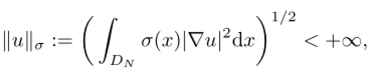
where σ is a nonnegative weighted function in（DN）.Then，the space（DN，σ）is given by

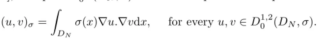
By［6，Lemma 3.1］，the space D1，20（DN，σ）is a Hilbert space with respect to the inner product

We denote by|.|mthe norm of Lm（DN）and|.|2=|.|for m=2.

The following lemma is a generalized version of the Poincar´e inequality；see［5］.

Lemma 2.1Let DNbe a bounded（resp.unbounded）domain of RN，N≥2 and assume that condition Hα（resp.Hβα）is satisfied.Then there eixsts a positive constant c such that

Remark 2.2It is pointed out in［5，6］that in the case of bounded case，（2.1）holds for α∈（0，2］；and the case α=2 can be considered as a“critical case”，that is to say，for α＞2 in（Hα）there exist functions such that（2.1）is not satisfied.Note that in the case of unbounded domain，inequality（2.1）generally does not hold if β≤2 in（Hβα）.

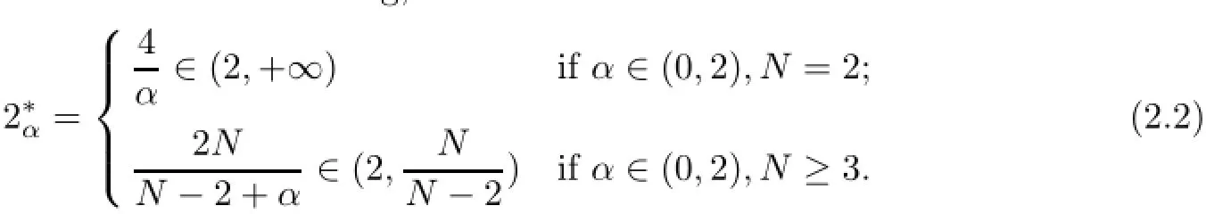
Let N≥2 and α∈（0，2）.We introduce the notation 2∗α，which has the role of the critical exponent in the classical Sobolev embedding，

As indicated in［5，6］，the following two lemmas demonstrate the continuous and compact inclusions of the space（DN，σ）L2（DN）.

Lemma 2.3Assume that DNis a bounded domain in RN，N≥2 and σ satisfies（Hα）. Then，the following embeddings hold：

Lemma 2.4Assume that DNis an unbounded domain in RN，N≥2 and σ satisfies）.Then，the following embeddings hold：

Remark 2.5Notethat if either condition（Hα）or（H）holds，the embedding（DN，σ）L2（DN）is compact.However，as σ is not in（DN），there is not in general any embedding relation between the space（DN，σ）and the standard Sobolev space H01（DN）.

We define a unbounded linear operator determined by the leading term in（1.1）

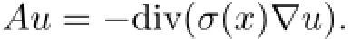
Under the conditions（Hα）or），the operator A is a positive and self-adjoint linear operator with domains defined as

which is a Hilbert space with respect to the usual graph scalar product.

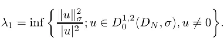
The eigenvectors of the operator A form the complete orthonormal familyin L2（DN）and the corresponding spectrum is discrete and denoted bysatisfying that

and

Furthermore，

3　Preliminaries on Random Dynamical Systems

Our aim is to describe problem（1.1）-（1.2）as a random dynamical system（RDS）.Thus，we need to recall some basic concepts and results related to the RDS.More information and detailed exposition can be found in［20-24］.

Let X be a separable Banach space with norm‖.‖Xand Borel σ-algebra B（X），that is，the smallest σ-algebra on X which contains all open subsets.

The basic notion in RDS is a measurable dynamical system（MDS）θ≡（Ω，F，P，（θt）t∈R），which is a probability space（Ω，F，P）combination with a group θt，t∈R，of measure preserving transformations of（Ω，F，P）such that probability measure P is ergodic and invariant with respect to θ.

Definition 3.1A RDS on X over a MDS θ is a family of measurable mappings

such that for P-a.e.ω∈Ω，the mappings ϕ satisfy the cocycle property：

for all s，t∈R+，x∈X.

Definition 3.2A random set｛D（ω）｝ω∈Ωis a family of subsets of X indexed by ω such that for every x∈X，the mapping ωd（x，D（ω））is measurable with respect to F，where for nonempty sets A，B∈2X，we set

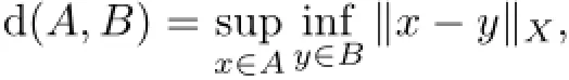
and in particular d（x，B）=d（｛x｝，B）.If further D（ω）is closed in X for every ω∈Ω，then｛D（ω）｝ω∈Ωis called a closed random set.

In the sequel，we denote by D a universe of the nonempty bounded random subsets of X. In particular，D satisfies the inclusion closed property.Namely，if D′（ω）⊂D（ω）for ω∈Ω and D=｛D（ω）｝ω∈Ω∈D，then D′=｛D′（ω）｝ω∈Ω∈D.

Definition 3.3Let D be a universe of sets.

（1）A random set｛K（ω）｝ω∈Ω∈D is a D-attracting for RDS ϕ if for P-a.e.ω∈Ω and every D∈D，

（2）A random set｛K（ω）｝ω∈Ω∈D is a D-random absorbing for RDS ϕ if for P-a.e.ω∈Ωand every D∈D，there exists a moment T=T（D，ω）＞0 such that for all t≥T，

Definition 3.4Let D be a universe of sets.A D-random attractor for RDS ϕ is a compact random set｛A（ω）｝ω∈Ω∈D satisfing that｛A（ω）｝ω∈Ωis a D-attracting set and ϕ（t，ω，A（ω））=A（θtω）for ω∈Ω and all t≥0.

Definition 3.5（［16］）Let D be a universe of sets.A RDS ϕ on X is said to be D-omegalimit compact if for P-a.e.ω∈Ω and for every D∈D，we have

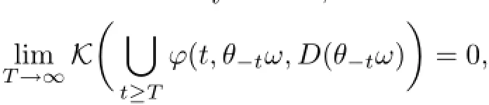
where K（B）is the Kuratowski measure of non-compactness of B defined by

K（B）=inf｛d＞0：B addmits a finite cover by sets of diameter≤d｝.

Definition 3.6（［16］）（i）A RDS ϕ is called to be continuous if the mappings ϕ：xϕ（t，ω，x）are continuous in X for all t∈R+，that is，norm-to-norm（briefly，norm）continuity.

（ii）A RDS ϕ on X is said to be norm-to-weak continuous if for P-a.e.ω∈Ω，

as n→+∞.

（iii）A RDS ϕ is called quasi-continuous if for P-a.e.ω∈Ω，

whenever（tn，xn）∈R×X is a sequence such that｛ϕ（tn，ω，xn）｝is bounded and（tn，xn）→（t，x）as n→+∞，where⇀means weak limit.

Remark 3.7Indeed，we can show that norm（resp.weak）continuity⇒norm-to-weak continuity⇒quasi-continuity.

Proposition 3.8（［16］）Let X，Y be two Banach spaces，X∗，Y∗be their dual spaces respectively.Assume that the embedding i：XY is densely continuous and its adjoint i∗：Y∗X∗is dense.If an RDS ϕ is continuous or norm-weak continuous in Y，then ϕ is quasi-continuous in X.

The following existence result on D-random attractor for an RDS can be found，for instance，in［16，25，26］.

Theorem 3.9Let D be a universe of set，which is inclusion closed.Suppose that ϕ is a quasi-continuous RDS on X.If there exists a closed and bounded D-random absorbing set｛K（ω）｝ω∈Ωfor ϕ on X and ϕ is D-omega-limit compact，then the random set｛A（ω）｝ω∈Ω，where A（ω）is structured by

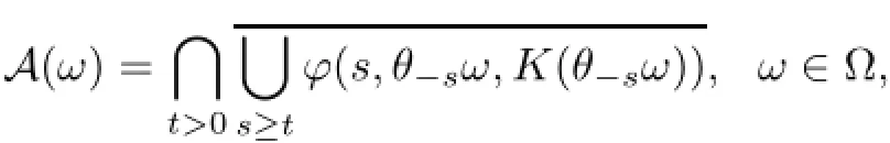
is a unique D-random attractor for ϕ in X.

4　Generation of Quasi-Continuous RDS

In this section，we will show the generation of a quas-continuous RDS of the equations

with the initial value and boundary condition where the non-linearity f（s）in（4.1）satisfies that for s∈R，

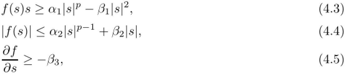
where αi（i=1，2）and βi（i=1，2，3）are positive constants and p＞2.The nonlinearity f is different from the one in［12］.As a typical model，f（s）=|s|p−2s satisfies all the conditions（4.3）-（4.5）.

We give the canonical probability space（Ω，F，P），where Ω=｛ω∈C（R，Rm）：ω（0）=0｝，F is the Borel σ-algebra induced by the compact-open topology of Ω，and P is the corresponding Wiener measure on（Ω，F）.Then，we identify W（t）with ω（t），Define the Wiener time shift operators by This shift θtis a group on Ω，which leaves the Wiener measure P invariant and ergodic.In particular，θ=（Ω，F，P，（θt）t∈R）is an ergodic MDS；see［20］.

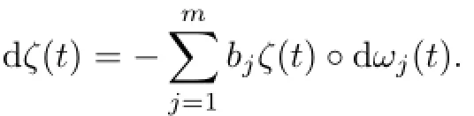
Consider the stochastic processthat satisfies the Stratonovich equation

Let u（t）be a solution to the initial problem（4.1）-（4.2）.Then，v（t）=ζ（t）u（t）solves the equation

with initial value condition

By a standard Faedo-Galerkin approximation technique，we can show that the problem（4.6）-（4.7）with g∈L2（DN）is well-posed in L2（DN）.In particular，for P-a.e.ω∈Ω，we have

Theorem 4.1Assume that f satisfies（4.3）-（4.5），g∈L2（DN），and vτ∈L2（DN），τ＜T.（i）Then，the problem（4.6）-（4.7）possesses a unique weak solution

（iii）Denoting such solution by v（t，ω；vτ）with initial value vτ，the mapping vτv（t，ω；vτ）is continuous in L2（DN）for all t≥τ.

Then，ϕ is a continuous RDS on L2（DN）over the MDS（Ω，F，P，and therefore by Proposition 3.8，ϕ is a quasi-continuous RDS onObviously，by（4.8）we deduce that

To obtain the existence of random attractors in some proper spaces，from（4.9）it is necessary to obtain the estimate of solution at the left neighbourhood of time at zero as the initial time−t goes to negative infinite.

5　Existence of Compact Random Attractor

Throughout this article，if DNis an unbounded domain，then we may assume that β1＜λ，where β1is in（4.3），and further we denote by γ=λ−β1.When DNis bounded，this assumption is not necessary and should be omitted，and in this case，we put γ=λ.

Let D be a universe of some families of non-empty random subsets of（DN，σ）such that

Note that ζ（t）is continuous and positive on［−2，0］.Then，there exist finite constants E，F＞0 such that

We first introduce an important lemma，which will be used in what follows.

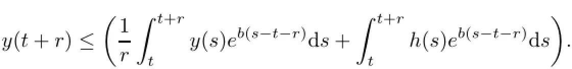
Lemma 5.1（［15］）Suppose that y and h are two nonnegative functions on［a，∞）such that y，and h are locally integrable.If for every t≥a，

then，for every r＞0，one has

5.1Asymptotic estimates of the solution

In this subsection，we will give the estimates for the solution in the spaces（DN，σ），Lp（DN）and L2p−2（DN），respectively.The number c is a positive constant depending only on the nonnegative numbers αi（i=1，2），βi（i=1，2，3），λ，p，E，F，and the norms|g|，|g|2p−2of the function g.

Lemma 5.2Assume that g∈L2（DN）∩L2p−2（DN）and f satisfies（4.3）-（4.5）.Then for P-a.e.ω∈Ω，the solution v（t，ω；ζ（τ）uτ）of equations（4.6）-（4.7）satisfies that for all t≥τ，

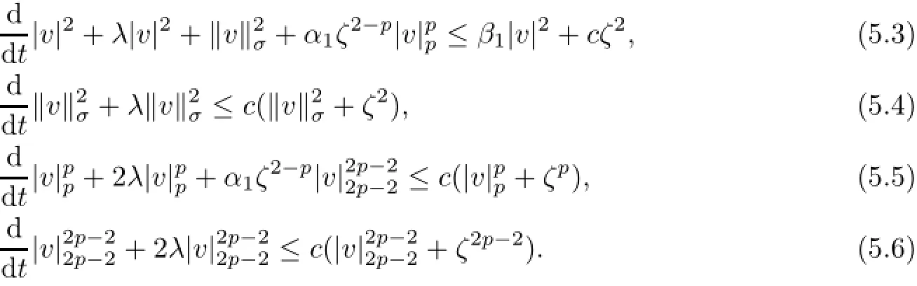
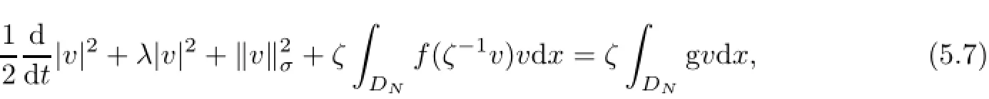
ProofTo prove inequality（5.3），we multiply（4.6）by v，and then integrate over DNto find that

where by（4.3），we have

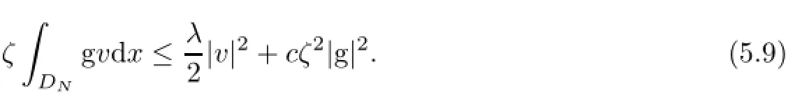
and by the ǫ-Young inequality， We combine（5.7）-（5.9）to obtain inequality（5.3）.

We then prove inequality（5.4）.To this end，we multiply（4.7）with Av and then integrate over DNto produce

where by（4.5），

and by ǫ-Young inequality，

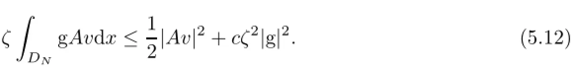
Then，inequality（5.4）is given by（5.10）-（5.12）.

To prove inequality（5.5），we multiply（4.6）by|v|p−2v and then integrate over DNto yield

We see that

By assumption（4.3），it is easy to get

from which，it follows that

In contrast，by the ǫ-Young inequality，we deduce that Thus，it follows from（5.13）-（5.14）and（5.16）-（5.17）that

from which and p≥2，we have showed（5.5）.

We finally prove inequality（5.6）.Multiplying（4.7）with v2p−3，we obtain

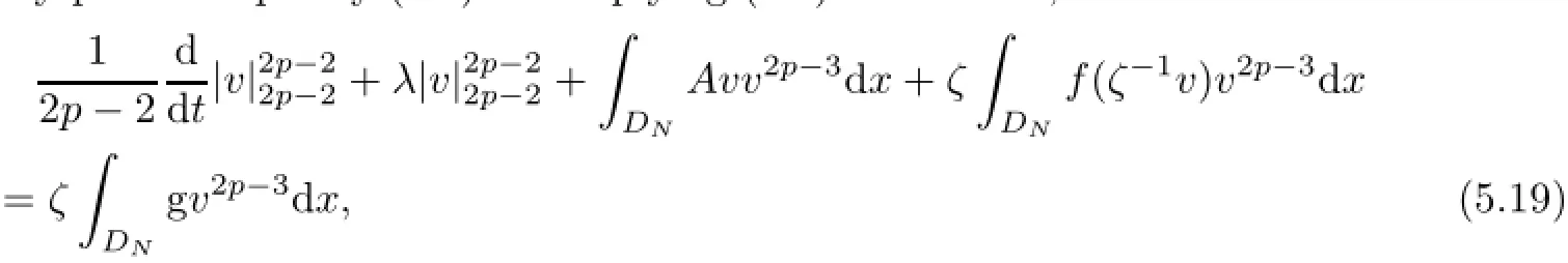
where

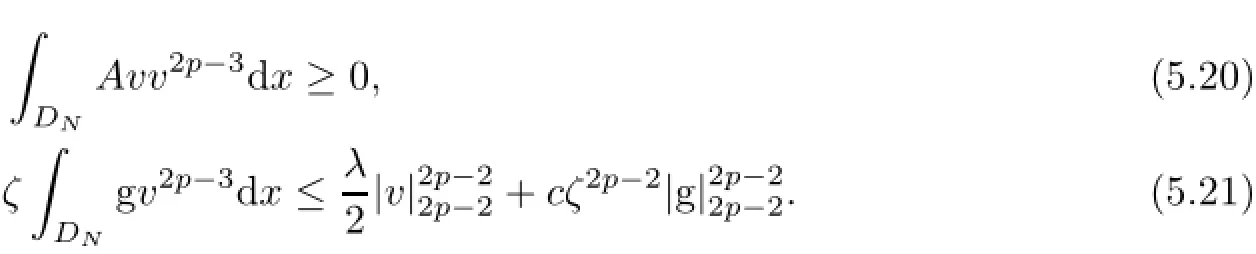
By（5.15），we have

Therefore，by（5.19）-（5.22），we get

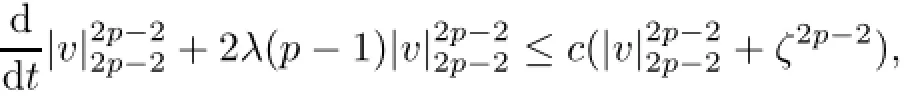
which proves（5.6）.

Lemma 5.3Assume that g∈L2（DN）∩L2p−2（DN）and f satisfies（4.3）-（4.5）.Let D be defined by（5.1）and D=｛D（ω）｝ω∈Ω∈D.Then，there exist positive variables1（ω）and2（ω）such that for P-a.e.ω∈Ω there exists T=T（D，ω）＜−2 such that for all τ≤T，the solution v（t，ω；ζ（τ）uτ）of equations（4.6）-（4.7）with uτ∈D（θτω）satisfies

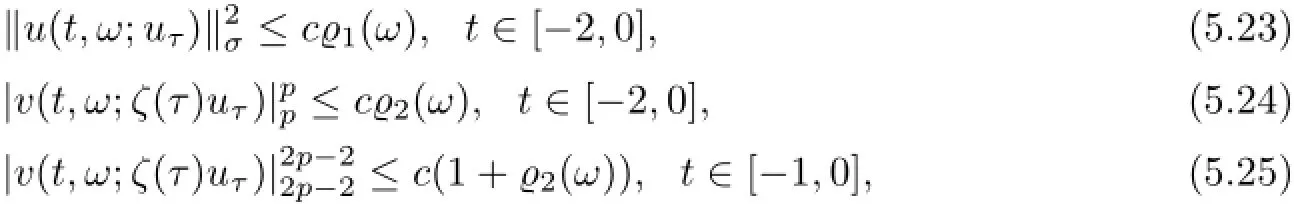
where v（t）=ζ（t）u（t）.

ProofWe first assume that DNis unbounded.Then，it follows from the energy inequality（5.4）and Lemma 5.1 that for t∈［−2，0］and τ＜−2，

where γ=λ−β1＜λ.To estimate the first term on the right-hand side of（5.26），we rewrite（5.3）as

We multiply both sides of（5.27）by eγt，and then integrate over the interval［τ，t］to yield

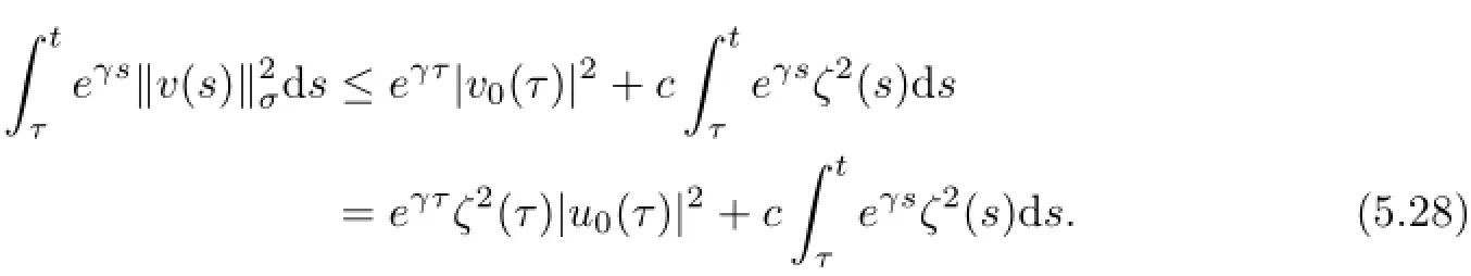
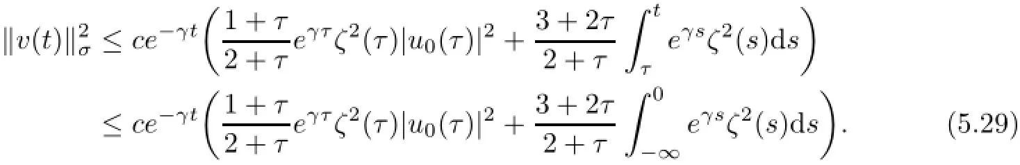
It follows from（5.26）and（5.28）that for every t∈［−2，0］and τ＜−2，

If DNis bounded，then by the embedding relation of Lp（DN）L2（D）and the inverse ǫ-Young inequality，we have

where η is the embedding constant.Thus，we can also obtain（5.27）with γ being replaced by λ，and then（5.29）is followed with γ=λ.Now，by standard argument（using，for example，the law of the iterated logarithm），seeing［22］，we have

Then，by（5.29）-（5.30）we find that for every uτ∈D（θτω），there exists T1=T1（D，ω）＜−2 such that for every τ≤T1and t∈［−2，0］，

where

This gives

which proves（5.23）.

We next prove estimate（5.24）.Using Lemma 5.1 to inequality（5.5），we get，for t∈［−2，0］and τ＜−2，

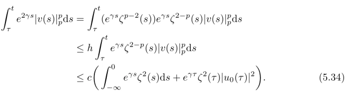
By（5.27）and a similar technique to the deriving of estimate of（5.28），we see that

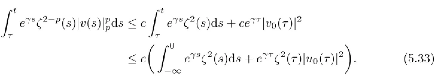
By the property of ζ（s），it is easy to show that there exists a constant h＞0 such that

which，along with（5.33），gives

Then，combination with（5.32）and（5.34），it infer that

which implies that for every uτ∈D（θτω），there exists T2=T2（D，ω）＜−2 such that for every τ≤T2and t∈［−2，0］，

where

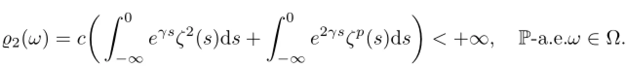
Finally，we show that（5.25）holds.By utilizing Lemma 5.1 to inequality（5.6）over the interval［−2，t］with t∈［−1，0］，we deduce

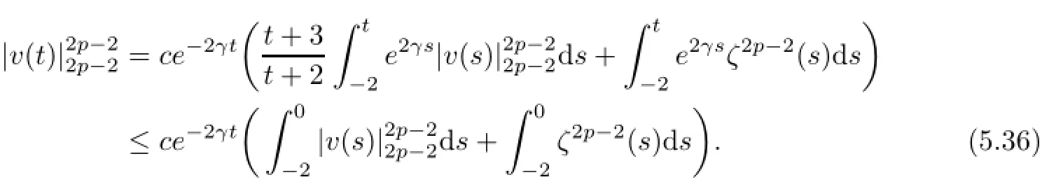
where we have used the facts that 0＜≤3 on［−1，0］and 0＜e2γs≤1 on［−2，0］.In contrast，we integrate（5.5）with respect to t over the interval［−2，0］to produce that，along with（5.35），

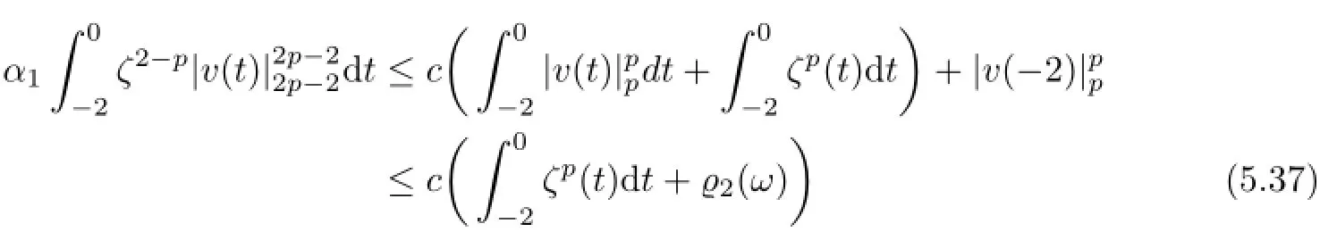
for all uτ∈D（θτω）and τ≤T2.Hence，by（5.2）and（5.37），we obtain

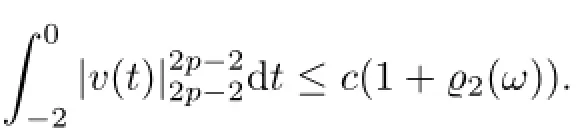
This，together with（5.36），yields

for every τ≤T2.Put T=min｛T1，T2｝.Then，we complete the proof.

In this subsection，we consider the existence of random attractor in（DN，σ）.The related idea is that there is a natural splitting of the weighted space（DN，σ）into a finitedimensional subspace and its infinite-dimensional orthogonal complement，such that solutions of the problem（4.1）-（4.2）is decomposed into two parts；one part of which is bounded in an m-dimensional subspace while the other one vanishes as m increases to infinity.

Let Hm=span｛e1，e2，···，em｝⊂（DN，σ）and Pm：（DN，σ）→Hmbe the canonical projector and I be the identity.As such，for every v∈（DN，σ），v has a unique decomposition：v=Pmv+vm，where

Lemma 5.4Assume that g∈L2（DN）∩L2p−2（DN）and f satisfies（4.3）-（4.5）.Let D be defined by（5.1）and D=｛D（ω）｝ω∈Ω∈D.Then，for P-a.e.ω∈Ω and every ε＞0，there are N=N（ω，ε）∈Z+and T=T（D，ω）＜−2 such that for all τ≤T and m≥N，the solution u（t，ω；ζ（τ）uτ）of the problem（4.1）-（4.2）with uτ∈D（θτω）satisfies

ProofFirst by assumption（4.4）we have

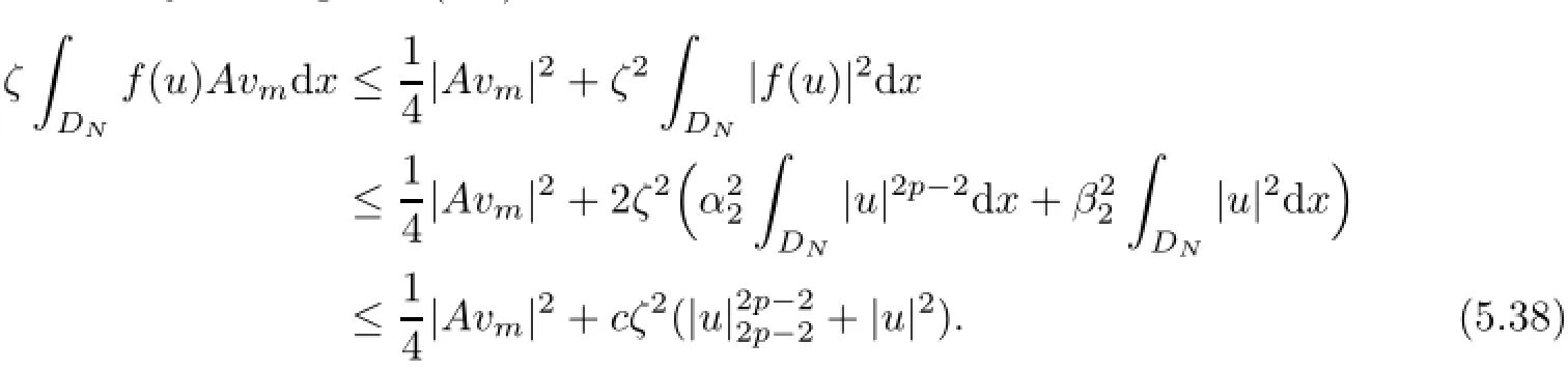
Then，we multiply（4.6）by Avmand integrate over DNto find that

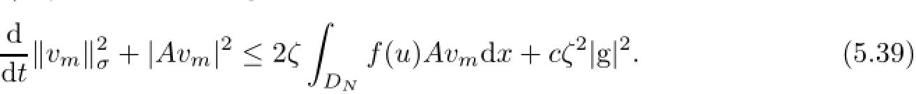
Hence，（5.38）and（5.39）imply that

By applying Lemma 5.1 to（5.40）over the interval［−1，0］to get

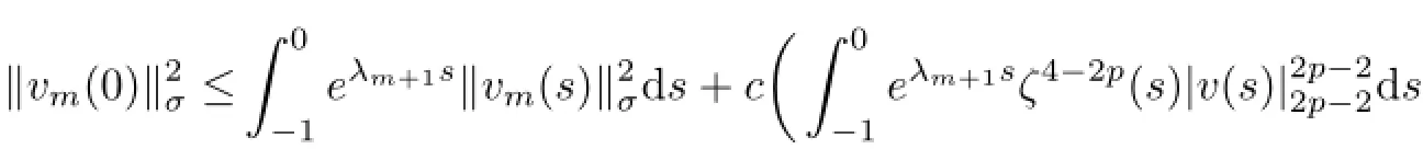
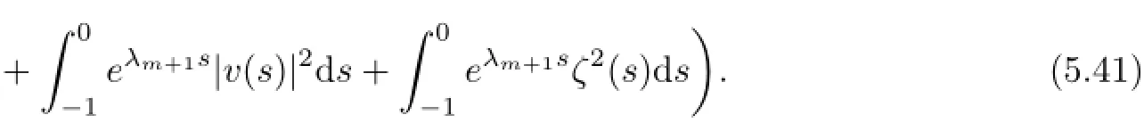
We estimate every terms on the right-hand side of（5.41）.By（5.23），there exists T=T（D，ω）＜−2 such that for every τ≤T，

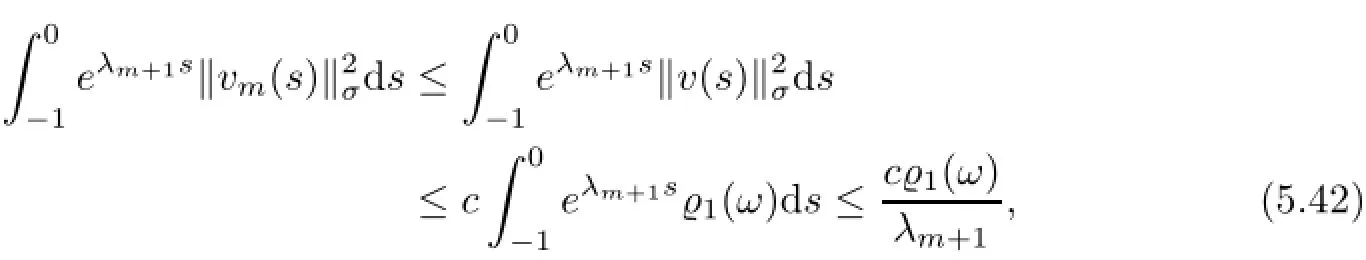
where and the following，we let T be in Lemma 5.3.By（5.2）and（5.25），the second term on the right-hand side of（5.41）is bounded by

for all τ≤T.Moreover，by the Poincar´e inequality in Lemma 2.1 and（5.23），the third term on the right-hand side of（5.41）is bounded by

for all τ≤T.The last term on the right-hand side of（5.41）is estimated by

Consequently，it follows from（5.41）-（5.44）that

Noting that λm+1increases to infinity as m→∞，we can choose N=N（ε，ω）∈Z+such that for all m≥N and τ≤T，

and thus，

for every uτ∈D（θτω）and m≥N and τ≤T.

Theorem 5.5Assume that g∈L2（DN）∩（DN）and f satisfies（4.3）-（4.5）.Then，the RDS ϕ associated with initial problem（4.1）-（4.2）admits a unique D-random attractorin（DN，σ），which attracts every random set belonging to D in the topology of（DN，σ）space.

ProofBy（4.9），there holds

Hence，using（5.23）at time t=0，it infers that for every u0（ω）∈D（ω），there exists a random constant T1=T1（D，ω）＞2 such that for all t≥T1，

which gives a D-random absorbing set defined by K0（ω）=｛u∈D1，20（DN，σ）；‖u‖2σ≤1（ω）｝，ω∈Ω.We need to show that1（ω）satisfies（5.1）.First，by the Poincar´e inequality（2.1）it follows that

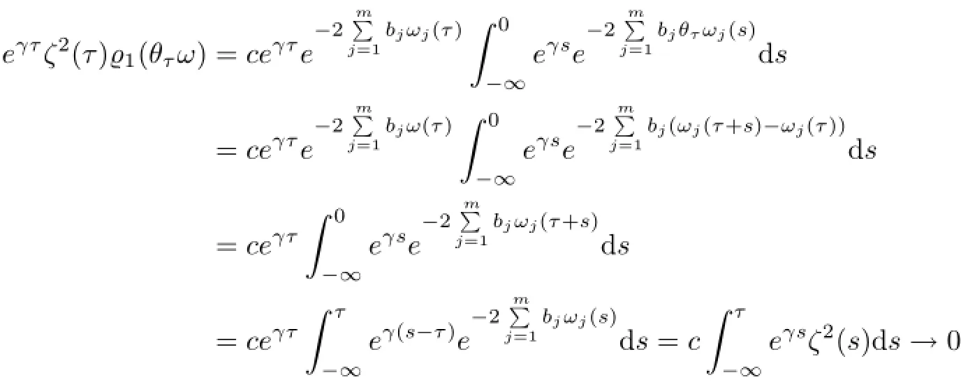
as τ→−∞.Hence，｛K0（ω）｝ω∈Ω∈D.By（5.45）we also have

where Pmis the projection operator.

In contrast，by Lemma 5.4，for every ε＞0，there are random constants N1=N1（ε，ω）∈Z+and T2=T2（D，ω）＞0 such that for all t≥T2and m≥N1，

We fix m=m0≥N1.Then，by utilizing the additive property of Kuratowski measure of non-compactness［16，Lemma 2.5（iii）］，it follows from（5.47）and（5.48）that for P-a.e.ω∈Ωand t≥T2，

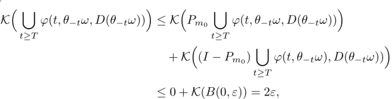
where B（0，ε）is the ε-neighborhood at centre 0 in（DN，σ）.This shows that the RDS ϕ generated by initial problem（4.1）-（4.2）is D-omega-limit compact.Hence，the conditions of Theorem 3.9 are all satisfied.The proof is completed.

5.3Random attractor in L（DN）（∈［2，2p−2］）

To study the existence of random attractors in L（DN）（∈［2，2p−2］），we first state some theorems and lemmas.By Theorem 5.5 and the continuous embedding of（DN，σ）L2（D），we immediately obtain the existence of random attractor｛A（ω）｝ω∈Ωin L2（DN）.

Theorem 5.6Assume that g∈L2（DN）∩L2p−2（DN）and f satisfies（4.3）-（4.5）.Then，the RDS ϕ associated with initial problem（4.1）-（4.2）admits a unique D-random attractor｛A（ω）｝ω∈Ωin L2（DN），where 2＜p＜+∞.

In the following，we consider the existence of random attractor in L（DN），where 2＜≤2p−2 with p＞2.We need some preliminaries.

Lemma 5.7（Interpolation inequality）If 0＜q≤≤r≤+∞and O is a bounded or unbounded domain in RN，then Lq（O）∩Lr（O）⊆L（O）and

The next theorem shows that if the RDS ϕ possesses a D-random attractor in L2，then the existence of random attractor in Ll（l＞2）is justified only under the condition that ϕ is D-omega-limit-compact in the topology of Ll.It seems that the existence of a random absorbing set in Llis not necessary；see［27］.For clarification，we give the skeleton of proof.

Theorem 5.8Let ϕ be a continuous RDS on L2and be a RDS on Llover the same MDS θ with ϕ（L2）⊆Ll，where 2＜l＜∞.Let D be a universe in L2which is included closed. Suppose that

（i）ϕ possesses a D-random absorbing set｛K（ω）｝ω∈Ωin L2；

（ii）ϕ is D-omega-limit-compact in the topology of L2and Ll，respectively.

Then，the family of random sets｛Al（ω）｝ω∈Ω，where

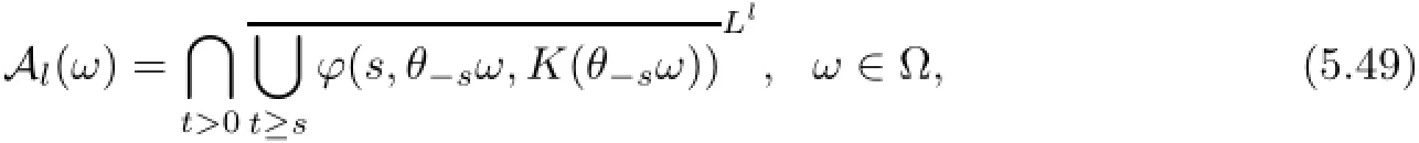
is a unique D-random attractor in Llin the sense that for P-a.e.ω∈Ω，

（a）Al（ω）is compact in Ll；

（b）ϕ（t，ω，Al（ω））=Al（θtω）；

（c）｛Al（ω）｝ω∈Ωis D-attracting in the topology of Ll.

Furthermore，Al（ω）=A（ω）for ω∈Ω，where｛A（ω）｝ω∈Ωis the D-random attractor in L2（DN）.

ProofStep one，compactness.By ϕ（L2）⊆Ll，the right-hand side of（5.49）makes sense. Because ϕ is D-omega-limit compactness of ϕ in Ll，by Lemma 4.5（v）in［16］），we have

Step two，invariance.By Theorem 2.5，there is an D-random attractor in L2which is denoted by｛A（ω）｝ω∈Ω，where

If we have showed that A（ω）=Al（ω）for ω∈Ω，where Al（ω）is in（5.49），then the invariant property is followed.To this end，according to（5.49）and（5.50）we give the following two equivalent relations：for ω∈Ω，

and

If x∈A（ω）for ω∈Ω，by the equivalence regime（5.51），there exist two sequences tn→∞and xn∈K（θ−tω）such that

Note that｛K（ω）｝ω∈Ω∈D and ϕ is D-omega-limit compact in Ll.Then，there exist an y∈Lland a subsequence｛nk｝with tnk→∞such that

and by［27，Lemma 2.7］，we have x=y，and therefore，x∈Al（ω）.That is to say，A（ω）⊆Al（ω）for ω∈Ω.The inverse inclusion relation can be proved by a similar argument and whereas A（ω）=Al（ω）for ω∈Ω.Hence，｛Al（ω）｝ω∈Ωpossesses the invariance property.

Step three，attracting.This is followed by a similar argument as［27，Lemma 2.8］.

The above criterion（ii）can be replaced by the following easy-to-check condition in a concrete RDS.The proof is similar to［27，Lemma 2.9］，so we omit it here.

Theorem 5.9Suppose that the RDS ϕ is D-omega-limit compact in L2，and for any ε＞0 and every D=｛D（ω）｝ω∈Ω∈D，there exist positive random constants c=c（ω），M= M（ε，D，ω），and T=T（D，ω）such that for all t≥T，

Then，ϕ is D-omega-limit compact in Ll.

To check the condition of Theorem 5.9，we denote

and

Lemma 5.10Assume that g∈L2（DN）∩L2p−2（DN）and f satisfies（4.3）-（4.5）.Let D be defined by（5.1）and D=｛D（ω）｝ω∈Ω∈D.Then，for P-a.e.ω∈Ω and every ε＞0，there exist random constants T=T（D，ω）＜−2，c=c（ω）＞0，and M=M（ε，D，ω）＞0 such that for all τ≤T，the solution v（t，ω；ζ（τ）uτ）with uτ∈D（θτω）satisfies

The idea of proof is from［28-30］.Here，we develop this method and do not need to check that the measure mes（DN（|u|≥M））≤ε and the estimateR DN（|v（t）|≥M）|v（t）|2dx≤ε，comparing to some similar studies as in［15，16，27，31］.

ProofPut t∈［−1，0］and M＞1.To obtain（5.54），we multiply（4.6）by（v−M）−1and then integrate over DNto get

where（v−M）+is positive part of v−M，that is，

We now estimate the terms of（5.55）.It is obvious that

If v≥M，then，by（5.2），u=ζ−1v≥F−1M＞0 for t∈［−1，0］，and hence by（4.3），

On the other hand，|v|p−1≥|v|p−2（v−M）≥Mp−2（v−M）holds on.Then，it follows that

where t∈［−1，0］and F is in（5.2）.The term on the right-hand side of（5.55）is estimated as

Combining（5.55）-（5.60），we obtain

where t∈［−1，0］and δ=δ（M）=α1Mp−2F2−pvaries only with M and the positive constant c is independent of M.We can use Lemma 5.1 over the interval［−1，t］and restriction on t∈［−1/2，0］to find that

According to（5.23）and（5.25），by employing Lemma 5.7 there exist random constants ρ（ω）and T1=T1（D，ω）＜−2 such that for every t∈［−1，0］，−1

−1for every uτ∈D（θτω）and τ≤T1.Furthermore，Because g∈L2（DN）∩L2p−2（DN），by Lemma 5.7 we also have≤C，where C is a positive non-random constant.Hence，combining（5.62） and（5.63），we find that

for every uτ∈D（θτω）and τ≤T1.As δ=α1Mp−2F2−pincreases as M→+∞，we can choose M=M1large enough such that for every t∈［−1/2，0］，

for every uτ∈D（θτω）and τ≤T1.

Consider that if v（t）≥2M1then v（t）−M1≥D1+⊃D2+.Then，it follows from（5.65）that for every t∈［−1/2，0］，

for every uτ∈D（θτω）and τ≤T1.

We exert the same arguments as（5.66），working with（v+M）−）−1instead of（v−M）−1+，where（v+M）−is the negative part of v+M，to deduce that there exists T2=T2（D，ω）＜−2 and M2=M2（ε，D，ω）large enough such that for every t∈［−1/2，0］，

for every uτ∈D（θτω）and τ≤T2.

Put T=min｛T1，T2｝.Then，（5.66）and（5.67）hold for all τ≤T.Write M=max｛M1，M2｝.

It follows from（5.66）and（5.67）that for all τ≤T，Z

for every uτ∈D（θτω）and t∈［−1/2，0］.This is the desired result.

By Theorem 5.6，Theorems 5.8-5.10，we immediately obtain

Theorem 5.11Assume that g∈L2（DN）∩L2p−2（DN）and f satisfies（4.3）-（4.5）.Then，the RDS ϕ generated by equations（4.1）-（4.2）has a unique random attractor｛A（ω）｝ω∈Ωin L（DN）which is a compact random set attracting every subset D∈D，whereis determined

Remark 5.12Indeed，we also have A0（ω）=A（ω）for every ω∈Ω and 2≤≤2p−2. Furthermore，they are all the omega-limit set of the D-random absorbing set｛K（ω）｝ω∈Ω.

References

［1］Dautray R，Lions J L.Mathematical Analysis and Numerical Methods for Science and Technology.Vol.I：Physical origins and classical methods.Berlin：Springer-Verlag，1985

［2］Eidus D，Kamin S.The filtration equation，in a class of functions decreasing at infinity.Proc Amer Math Soc，1994，120（3）：825-830

［3］Gurtin M E，Macamy R C.On the Diffusion of biological populations.Math Biosci，1977，33：35-49

［4］Murray J D.Mathematical Biology，II：Spatial Models and Biomedical Applications.New York：Springer-Verlag，2003

［5］Karachalios N I，Zographopoulos N B.On the dynamics of a degenerate parabolic equation：Global bifurcation of stationary states and convergence.Calc Var Partial Differential Equations，2006，25（3）：361-393

［6］Caldiroli P，Musina R.On a variational degenerate elliptic problem.Nonlinear Differ Equ Appl，2000，7（2）：187-199

［7］Anh C T，Bao T Q.Pullback attractors for a non-autonomous semi-linear degenerate parabolic equation. Glasgow Math J，2010，52（3）：537-554

［8］Anh C T，Hung P Q.Global existence and long-time behavior of solutions to a class of degenerate parabolic equations.Ann Polon Math，2008，93（3）：217-230

［9］Anh C T，Chuong N M，Ke T D.Global attractors for the m-semiflow degenerated by a quasilinear degenerate parabolic equation.J Math Anal Appl，2010，363（2）：444-453

［10］Niu W S.Global attractors for degenerate semilinear parabolic equations.Nonl Anal，2013，77：158-170

［11］Feireisl E，Laurencot P，Simondon F.Global attractors for degenerate parabolic equations on unbounded domains.J Differential Equations，1996，129（2）：239-261

［12］Yang M H，Kloeden P E.Random attractors for stochastic semi-linear degenerate parabolic equations. Nonlinear Analysis：Real World Applications，2011，12（5）：2811-2821

［13］Anh C T，Bao T Q，Thanh N V.Regularity of random attractors for stochastic semilinear degenerate parabolic equations.Electronic Journal of Differential Equations，2012，207：1-22

［14］Yin J Y，Li Y R，Zhao H J.Random attractors for stochastic semi-linear degenerate parabolic equations with additive noise in Lq.Appl Math Compu，2013，225（1）：526-540

［15］Zhao W Q.Regularity of random attractors for a stochastic degenerate parabolic equation driven by additive noises.Appl Math Compu，2014，239C（15）：358-374

［16］Li Y R，Guo B L.Random attractors for quasi-continuous random dynamical systems and applications to stochastic reaction-diffusion equations.J Differential Equations，2008，245（7）：1775-1800

［17］Guo B L，Guo C X，Pu X K.Random attractors for a stochastic hydrodynamical equation in Heisenberg paramagnet.Acta Mathematica Scientia，2011，31B（2）：529-540

［18］Zhao W Q.H1-random attractors for stochastic reaction diffusion equations with additive noise.Nonlinear Anal，2013，84：61-72

［19］Zhao W Q.H1-random attractors and random equilibria for stochastic reaction diffusion equations with multiplicative noises.Comm Nonlinear Sci Numer Simulat，2013，18（10）：2707-2721

［20］Arnold L.Random Dynamical System.Berlin：Springer-Verlag，1998

［21］Chueshov I.Monotone Random Systems Theory and Applications.Berlin：Springer-Verlag，2002

［22］Crauel H，Debussche A，Flandoli F.Random attractors.J Dynam Diff Equa，1997，9（2）：307-341

［23］Crauel H，Flandoli F.Attractors for random dynamical systems.Probab Theory Related Fields，1994，100（3）：365-393

［24］Schmalfuß B.Backward cocycle and attractors of stochastic differential equations//Reitmann V，Riedrich T，Koksch N.International Seminar on Applied Mathematics-Nonlinear Dynamics：Attractor Approximation and Global Behavior.Dresden：Technische Universitüat，1992：185-192

［25］Bates P W，Lu K N，Wang B X.Random attractors for stochastic reaction-diffusion equations on unbounded domains.J Differential Equations，2009，246（2）：845-869

［26］Flandoli F，Schmalfuß B.Random attractors for the 3D stochastic Navier-Stokes equation with multiplicative noise.Stoch Stoch Rep，1996，59（1/2）：21-45

［27］Zhao W Q，Li Y R.（L2，Lp）-random attractors for stochastic reaction-diffusion equation on unbounded domains.Nonlinear Anal，2012，75（2）：485-502

［28］Temam R.Infinite-Dimensional Dynamical Systems in Mechanics and Physics.New York：Springer-Verlag，1997

［29］Robinson J C.Infinite-Dimensional Dyanmical Systems：An Introduction to Dissipative Parabolic PDEs and the Theory of Global Attractors.Cambridge University Press，2001

［30］Zhong C K，Yang M H，Sun C Y.The existence of global attractors for the norm-to-weak continuous semigroup and its application to the nonlinear reaction-diffusion equations.J Differential Equations，2006，223（2）：367-399

［31］Li J，Li Y R，Wang B.Random attractors of reaction-diffusion equations with multiplicative noise in Lp. Appl Math Compu，2010，215（9）：3399-3407

March 9，2014；revised August 7，2014.This work was supported by China NSF（11271388），Scientific and Technological Research Program of Chongqing Municipal Education Commission（KJ1400430），and Basis and Frontier Research Project of Chongqing（cstc2014jcyjA00035）.