张 斌 吕 朵 段重阳 陈平雁△

1.3 多样本的均数比较

1.3.1 差异性检验

1.3.1.1 One-way ANOVA

方法:O'Brien和 Muller(1993)〔2〕给出的 One-way ANOVA样本量估计是建立在自由度为G-1，N-G，非中心参数为N·V/σ2的非中心F分布上。其检验效能的计算公式为:

在计算样本量时，一般先设定样本量初始值，然后迭代样本量直到所得的检验效能满足条件为止。此时的样本量，即研究所需的样本量。

【例1－22】一项有关降血压药的临床试验，设置3个处理组，即安慰剂、阳性对照药和新药，以舒张压下降值为主要疗效评价指标。由以往研究结果获知，安慰剂可使舒张压平均下降5mmHg，阳性对照药可下降12mmHg，公共标准差为6mmHg。我们预期新药的效果与阳性对照药相当，即可使舒张压下降12mmHg。若设定检验效能为90%，试估计样本量。

nQuery Advisor 7.0实现:设定检验水准 α=0.05;检验效能取1－β=90% 。依据上述基础数据可知，μ1=5，μ2=12，μ3=12，σ =6。在 nQuery Advisor 7.0主菜单选择:

Goal:Make Conclusion Using:⊙Means

Number of Groups:⊙ ＞ Two

Analysis Method:⊙Test

方法框中选择:One-way analysis of variance。

Assistants:⊙Compute Effect Size

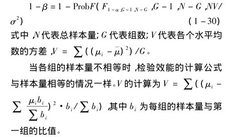
在弹出的标准差计算窗口将各参数键入，如图1－52所示，结果为V=10.899。

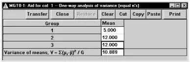
图1－52 nQuery Advisor 7.0关于例1-22样本量估计的参数计算结果

将计算结果V和其他参数键入样本量计算窗口，如图1－53所示，结果为n=15。

图1－53 nQuery Advisor 7.0关于例1-22样本量估计的参数设置与计算结果

SAS9.2软件实现:

%let u={5 12 12};

%let r={1 1 1};PROC IML;

start MGT0(a，G，sd，power);error=0;

if(a＞1|a＜0)then do;error=1;print“error”“Test significance level must be in 0-1”;end;

if(sd ＜0)then do;error=1;print“error”“standard deviation must be ＞ =0”;end;

if(G＜0|ceil(G)^=G)then do;error=1;print“error”“The Number of groups must be positive integer”;end;

if(power＞100|power＜1)then do;error=1;print“error”“Power(%)must be in 1-100”;end;

if(error=1)then stop;

if(error=0)then do;

V=sum((＆u-sum(＆u#＆r/sum(＆r)))##2#＆r/sum(＆r));es=V/sd##2;total=G+1;

do until(pw＞=power/100);ncp=total*es;df1=G-1;df2=total-G;f=FINV(1-a，df1，df2);

pw=1-PROBF(f，df1，df2，ncp);total=total+0.01;end;

total=ceil(total-0.01);n=ceil(total/G);

print a［label=“Test significance level”］

G［label=“Number of groups”］

V［label=“Variance of means”］

sd［label=“Common standard deviation”］

es［label=“Effect size”］

power［label=“Power(%)”］

n［label=“n per group”］;end;

finish MGT0;

run MGT0(0.05，3，6，90);quit;

SAS运行结果:

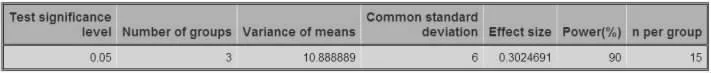
图1－54 SAS9.2关于例1-22样本量估计的参数设置与计算结果

式中，C代表每组的样本均数和对应对比系数的乘积的和，即∑μici;D=∑c2i;G为组数;σ为样本标准差。

当各组的样本量相等时，检验效能的计算公式与样本量不相等的情况一样，但每一组的对比系数应都为1。

在计算样本量时，一般先设定样本量初始值，然后迭代样本量直到所得的检验效能满足条件为止。此时的样本量，即研究所需的样本量。

【例1－23】接例22实验设计将安慰剂组、低剂量新药组、高剂量新药组与标准降血压药进行比较。我们估计安慰剂组的血压会有5mmHg的下降，标准药组下降 12mmHg，低剂量和高剂量分别下降10.5mmHg和13.5mmHg。我们再估计血压的标准差为6mmHg。为了保证足够的样本量，我们假设每组的标准差都为6mmHg。本研究若在90%的检验效能条件下，试估计样本量。

仍然是有关降血压药的临床试验，设置4个处理组，即安慰剂、阳性对照药、低剂量新药组和高剂量新药组，以舒张压下降值为主要疗效评价指标。由以往研究结果获知，安慰剂可使舒张压平均下降5mmHg，阳性对照药可下降12mmHg。由预试验得到的数据显示，低剂量新药和高剂量新药分别使舒张压下降10.5mmHg和 13.5mmHg。假定公共标准差为6mmHg，若设定检验效能为90%，试估计样本量。

nQuery Advisor 7.0实现:设定检验水准 α=0.05;双侧检验，即 s=2;检验效能取1－β=90% 。依据上述基础数据估计，μ1=5，μ2=10.5，μ3=13.5，μ4=12，σ=6，。在nQuery Advisor 7.0主菜单选择:

Goal:Make Conclusion Using:⊙Means

Number of Groups:⊙ ＞ Two

Analysis Method:⊙Test

方法框中选择:Single One-way between means contrast。

Assistants:⊙Compute Effect Size

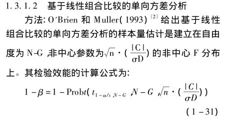
在弹出的标准差计算窗口将各参数键入，如图1－55所示，结果为C=3，D=1.414。将计算结果传输至主对话框，如图1－56所示，结果为n=85。

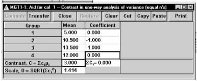
图1－55 nQuery Advisor 7.0关于例1-23样本量估计的参数计算结果

图1－56 nQuery Advisor 7.0关于例1-23样本量估计的参数设置与计算结果

SAS9.2软件实现:

%let u={5 10.5 13.5 12};

%let coe={0-1 1 0};

%let r={1 1 1 1};

proc IML;

start MGT1(a，s，G，sd，power);error=0;

if(a＞1|a＜0)then do;error=1;print“error”“Test significance level must be in 0-1”;end;

if(s^=1 ＆ s^=2)then do;error=1;print“error”“s=1 or 2”;end;

if(sd ＜0)then do;error=1;print“error”“Standard deviation must be ＞ =0”;end;

if(G＜0|ceil(G)^=G)then do;error=1;print“error”“The Number of groups must be positive integer”;end;

if(power＞100|power＜1)then do;error=1;print“error”“Power(%)must be in 1-100”;end;

if(sum(＆coe)^=0)then do;error=1;print“error”“The sum of coe must be 1”;end;

if(error=1)then stop;

if(error=0)then do;

C=sum(＆u#＆coe);D=sqrt(sum(＆coe##2/＆r));

es=abs(C)/(sd#D);n=2;*n of group 1;

do until(pw ＞ =power/100);total=n#sum(＆r);*the total N;ncp=n#es##2;df1=1;df2=total-G;if(s=2)then do;f1=finv(a，df1，df2);f2=finv(1-a，df1，df2);

pw=probf(f1，df1，df2，ncp)+1-probf(f2，df1，df2，ncp);

end;if(s=1)then do;f=finv(1-2*a，df1，df2);

pw=1-probf(f，df1，df2，ncp);

end;n=n+0.01;end;

n=ceil(n-0.01);

print a［label=“Test significance level”］

s［label=“1 or 2 sided test”］

G［label=“Number of groups”］

sd［label=“Common standard deviation”］

es［label=“Effect size”］

power［label=“Power(%)”］

n［label=“n per group”］;end;

finish MGT1;

run MGT1(0.05，2，4，6，90);quit;

SAS运行结果:

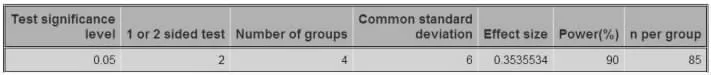
图1－57 SAS9.2关于例1-23样本量估计的参数设置与计算结果

1.3.1.3 双因素方差分析

方法:根据O'Brien和 Muller(1993)〔2〕提出的方法，双因素方差分析要考虑两个因素及其交互项对样本量的影响。而知道任何一个因素的检验效能可以计算另一个因素及交互因素的检验效能。各个因素检验效能的估计是建立在各自的自由度及非中心参数的F分布。其各自检验效能的计算公式为:

此时的μi是A因素某个水平下B因素的均数;μj是B因素某个水平下A因素的均数;μij是某个水平某个因素的均数;¯μ是所有数据的均数。

在计算样本量时，一般先设定样本量初始值，然后迭代样本量直到所得的检验效能满足条件为止。此时的样本量，即研究所需的样本量。

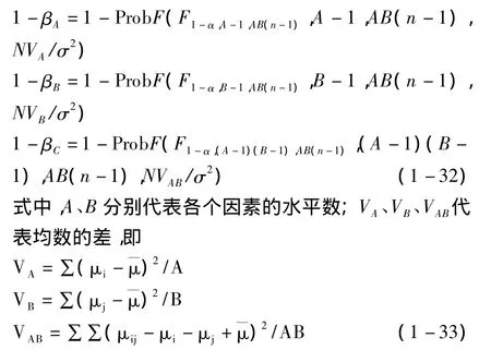
【例1－24】一项临床试验旨在评价两种作用于心脏收缩的新药控制收缩压的疗效，采用2×3析因设计，考虑两个因素:一个是性别(因素 A)，有男、女2个水平;另一个是药物(因素B)，有3个水平，分别是新药C、新药D和阳性对照药，评价指标为收缩压水平，详细背景见文献〔17〕。预实验数据显示:男性服用新药C、新药D和阳性对照药的平均收缩压分别为130mmHg、128mmHg、125mmHg;而女性服用新药 C、新药D和阳性对照药的平均收缩压分别为125mmHg、121mmHg、118mmHg;估计标准差为6 mm-Hg。采用平衡设计，设定药物间的检验效能为90%，试估计样本量。

nQuery Advisor 7.0实现:设定检验水准 α=0.05;检验效能取1-βB=90% 。由题意可知，μ11=130，μ12=128，μ13=125，μ21=125，μ22=121，μ23=118，σ=6;

在nQuery Advisor 7.0主菜单选择:

Goal:Make Conclusion Using:⊙Means

Number of Groups:⊙ ＞Two

Analysis Method:⊙Test

方法框中选择:Two-way analysis of variance。

Assistants:⊙Compute Effect Size

在弹出的计算窗口将各参数键入，如图1－58所示，结果为 VA=10.028、VB=6.000、VAB=0.222。将计算结果V传输至主对话框，键入其他参数后求得n=14(图1－59)。

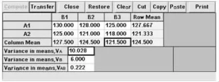
图1－58 nQuery Advisor 7.0关于例1-24样本量估计的参数计算结果

图1－59 nQuery Advisor 7.0关于例1-24样本量估计的参数设置与计算结果

SAS9.2软件实现:

%let means={130 128 125，125 121 118};

PROC IML;

start MGT2(a，lA，lB，sd，Apower，Bpower，AB-power);error=0;

if(a＞1|a＜0)then do;error=1;print“error”“Test significance level must be in 0-1”;end;

if(sd ＜0)then do;error=1;print“error”“Standard deviation must be ＞ =0”;end;

if(lA＜0|ceil(lA)^=lA)then do;error=1;print“error”“The number of factor A levels must be positive integer”;end;

if(lB＜0|ceil(lB)^=lB)then do;error=1;print“error”“The number of factor A levels must be positive integer”;end;

if(error=1)then stop;

if(error=0)then do;

*compute V;Va=sum((＆means［，:］-＆means［:］)##2)/lA;Vb=sum((＆means［:，］-＆means［:］)##2)/lB;Vab=sum((＆means-＆means［:］)##2)/(lA#lB)-Va-Vb;*interaction;

Aes=Va/(sd##2);Bes=Vb/(sd##2);ABes=Vab/(sd##2);

n=2;*n of every group;

do until(Apw＞=Apower/100＆Bpw＞=Bpower/100＆ABpw＞=ABpower/100);total=n*lA*lB;*the total N;df=lA*lB*(n-1);Ancp=total*Aes;dfa=lA-1;fa=finv(1-a，dfa，df);

Apw=1-probf(fa，dfa，df，Ancp);Bncp=total*Bes;dfb=lB-1;fb=finv(1-a，dfb，df);

Bpw=1-probf(fb，dfb，df，Bncp);ABncp=total*ABes;dfab=(lA-1)*(lB-1);fab=finv(1-a，dfab，df);

ABpw=1-probf(fab，dfab，df，ABncp);n=n+0.01;end;

n=ceil(n-0.01);total=ceil(total);

Apw=100*Apw;Bpw=100*Bpw;ABpw=100*ABpw;

print a［label=“Test significance level”］

lA［label=“Number of factor A levels”］

lB［label=“Number of factor B levels”］

Va［label=“Variance in means，VA”］

Vb［label=“Variance in means，VB”］

Vab［label=“Variance in means，VAB”］

sd［label=“Common standard deviation”］

Apw［label=“Power for A(%)”］

Bpw［label=“Power for B(%)”］

ABpw［label=“Power for AB(%)”］

n［label=“n per group”］;end;finish MGT2;

run MGT2(0.05，2，3，6，0，90，0);quit;

SAS运行结果:

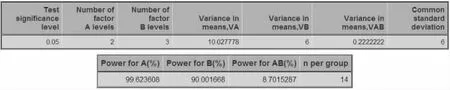
图1－60 nQuery Advisor 7.0关于例1-24样本量估计的参数设置与计算结果

致谢 我们在此感谢nQuery Advisor软件全球供销商“爱尔兰Statistical Solutions有限公司”为本研究提供的支持和帮助。

1．Elashoff JD．nQuery Advisor User's Guide．Ireland:Statistical Solutions Ltd．，2007．

2．O'Brien RG，Muller KE．Applied analysis of variance in behavioral science．New York:Marcel Dekker，1993:297-344．

3．Dixon WJ，Massey FJ．Introduction to Statistical Analysis．4th Edition．New York:McGraw-Hill，1983．

4．Overall JE，Doyle SR．Estimating sample sizes for repeated measures designs．Controlled Clinical Trials，1994，15:100-123．

5．Muller KE，Barton CN．Approximate power for repeated-measures ANOVA lacking sphericity．Journal of the American Statistical Association，1989，84:549-555．

6．Machin D，Campbell MJ．Statistical Tables for Design of Clinical Tri-als．Oxford:Blackwell Scientific Publications，1987．

7．Moser BK，Stevens GR，Watts CL．The two-sample t test versus satterthwaite approximate F test．Commun．Statist．-Theory Meth，1989，18:1963-3975．

8．Diletti E，Hauschke D，Steinijans VW．Sample size determination for bioequivalence assessment by means of confidence intervals．Int．Journal of Clinical Pharmacology，1991:29．

9．Noether GE．Sample size determination for some common nonparametric statistics．Journal of the American Statistical Association，1987，82:645-647．

10．Kolassa J．A comparison of size and power calculations for the Wilcoxon statistic for ordered categorical data．Statistics in Medicine，1995，14:1577-1581．

11．Senn S．Cross-over Trials in Clinical Research(2nd Edition)．New York:Wiley，2002．

12．Schuirmann DJ．A comparison of the two one-sided tests procedure and the power approach for assessing the equivalence of average bioavailability．Journal of Pharmacokinetics and Biopharmaceutics，1987，15:657-680．

13．Phillips KE．Power of the two one-sided tests procedure in bioequivalence．Journal of Pharmacokinetics and Biopharmaceutics，1990，18:137-143．

14．Owen DB．A special case of a bivariate non-central t-distribution．Biometrika 1965，52:437-446．

15．Chow SC，Liu JP．Design and Analysis of Bioavailability and Bioequivalence Studies．New York:Marcel Dekker，Inc．，1992．

16．Hauschke D，Kieser M，Diletti E，Burke M．Sample size determination for proving equivalence based on the ratio of two means for normally distributed data．Statistics in Medicine，1999，18:93-105．

17．SASInstitute，Inc．Getting Started with the SAS Power and Sample Size Application．North Carolina:SAS Institute，Inc．，2004．