Lin Xiaohan ,Liu Yuan,* ,Chen Fangjiong ,Huang Yang ,Ge Xiaohu

1 School of Electronic and Information Engineering,South China University of Technology,Guangzhou 510641,China

2 Key Laboratory of Dynamic Cognitive System of Electromagnetic Spectrum Space,Ministry of Industry and Information Technology,Nanjing University of Aeronautics and Astronautics,Nanjing 210016,China

3 School of Electronic Information and Communications,Huazhong University of Science and Technology,Wuhan 430074,China

Abstract: As a mature distributed machine learning paradigm,federated learning enables wireless edge devices to collaboratively train a shared AI-model by stochastic gradient descent (SGD).However,devices need to upload high-dimensional stochastic gradients to edge server in training,which cause severe communication bottleneck.To address this problem,we compress the communication by sparsifying and quantizing the stochastic gradients of edge devices.We frist derive a closed form of the communication compression in terms of sparsifciation and quantization factors.Then,the convergence rate of this communicationcompressed system is analyzed and several insights are obtained.Finally,we formulate and deal with the quantization resource allocation problem for the goal of minimizing the convergence upper bound,under the constraint of multiple-access channel capacity.Simulations show that the proposed scheme outperforms the benchmarks.

Keywords: federated learning;gradient compression;quantization resource allocation;stochastic gradient descent(SGD)

I.INTRODUCTION

As the boom of smart mobile devices,abundant data is produced at the network edge.Motivated by the valuable data and progressive artifciial intelligence (AI)algorithms,intelligent applications tremendously enhance productivity and effciiency in people’s daily lives.The transfer of the processing platform from the centralized datacenters in cloud to the user side in network edge boosts the development of edge AI or edge intelligence[1-6].

The movement of data processing from cloud to edge is highly non-trivial.To be specifci,cloud AI focuses on processing data under given aggregated global data.The central server needs to acquire local data from distributed edge devices via wireless links,and thus there inevitably exists a big challenge:transmitting tremendous amounts of data through radio access network (RAN) raises high costs,such as delay and energy consumption.In this case,wireless communication becomes the bottleneck of edge intelligence.Besides,the personal privacy may be violated when uploading raw data.Federated learning is a popular distributed machine learning pattern,where edge devices cooperatively train a shared AI model and local data is prevented from leaving edge devices [7-9].In particular,edge devices train their local models based on local datasets,and the local models/gradients are uploaded to edge server.Edge server use these local gradients to update the global model,and new global model is broadcast to edge devices for their local training.This server-device exchange is repeated until a certain level of global model accuracy is maintained.

However,the server-device exchange leads to severe communication bottleneck.The reason is that the trained models are usually high-dimensional while the radio resource is scare and the edge devices are capability-limited.Therefore,the gradients/models need to be compressed before transmission to reduce communication overhead.In addition,the channel conditions are time-varying and various across devices,so the compression needs to be adaptive to channel conditions.The above observations motivate us to study joint gradient compression and design a quantization resource allocation scheme.

1.1 Related Works

Federated learning can be studied by stochastic gradient descent (SGD) algorithm [7,10].In practice,stochastic gradients contain several high-dimensional vectors or arrays,which need large amounts of communication resources.To deal with this issue,two methods are developed to compress stochastic gradient.The frist is sparsifciation [11,12].After sparsifciation,only elements larger than the predefnied threshold are remained and uploaded.In [13,14],digital-distributed SGD(D-DSGD)method with coding and analog-distributed SGD (A-DSGD) method based on signal superposition are applied.In [15],momentum correction and local gradient clipping are jointly applied to promote model accuracy after sparsifciation.The second method is quantization,in which the single component or blocks of gradients are quantized to codes.For example,the authors in [16]studies a kind of scalar quantization method,quantized SGD(QSGD),where vector components are uniformly quantized.It is proved that QSGD makes a compromise between quantization variance and model accuracy.One-bit quantization and signSGD belongs to scalar quantization,in which the momentum in descent also achieve excellent performance compared with its counterpart [17,18].In [19],the Terngrad method quantizes the positive,negative and zero elements of gradients to be +1,-1 and 0,respectively.The authors in [20] use low dimensional Grassmannian manifolds to reduce the dimension of local model gradient.In [21],the local model update is compressed by dimension reduction and vector quantization.In [22],the authors focus on model compression during the training in federated learning,where a layered ternary quantization method is used to compress local model networks and different quantization thresholds are used in different layers.

Another feild of federated learning is the resource allocation optimization.In [23],edge devices upload their local models to BS via frequency domain multiple access(FDMA).The bandwidth allocation,transmit power,local computation frequency and communication time are jointly optimized to enhance energy effciiency.[24]provides a comprehensive research on the correlation between training performance and the effect of wireless network,measured by the packet error rate.The resource allocation and user selection are jointly optimized to minimize the training loss subject to the delay and energy consumption constraints.In [25],authors design a broadband analog aggregation scheme via over-the-air computation and study the communication-learning tradeoff.The authors in[26]present the federated learning scheme with overthe-air computation,and jointly optimize device selection and beamforming design.This problem is modeled as a sparse and low-rank optimization.The authors in [27] consider the federated learning over a multiple access channel(MAC)and optimize the local gradient quantization parameter.In [28],the quantization error and the channel fading are characterized in terms of received signal-to-noise ratio (SNR) and quantization resource allocation is studied.The authors in [29] propose a time-correlated sparsifciation method with hybrid aggregation(TCS-H),and jointly optimize the model compression and over-the-air computation to minimize the number of required communication time slots.The energy consumption of local computing and wireless communication are balanced in [30] by optimizing gradient sparsifciation and the number of local iterations.Adaptive Top-k SGD is proposed in [31] to minimize the convergence error under the constraint of communication cost.Rand-k sparsifciation and stochastic uniform quantization are considered in[32].

1.2 Contributions and Organization

This paper addresses the problem of communication compression in federated learning.We use sparsifciation and quantization jointly for local gradient compression to relieve communication bottleneck.We derive a closed form of the communication compression with respect to the sparsifciation and quantization parameters.Note that gradient compression results in information loss and thus distorts the training performance.Therefore,we study quantization resource allocation to minimize convergence upper bound by optimizing quantization levels of devices.The main contributions of this paper are summarized as follows.

•Closed-Form Communication Compression.We derive a closed-form communication compression in terms of sparsifciation and quantization factors,and the correlation between the two factors is analyzed mathematically.It is shown that sparsifciation and quantization are complementary for communication compression.

•Convergence Rate Analysis.We derive the upper bound of the convergence rate under joint sparsifciation and quantization.Several useful insights are found via our analysis: i)The proposed scheme converges as the growth of the number of device-server iterations;ii) When the number of devicesKbecomes larger,the convergence rate approacheswhereMis the number of device-server iterations.iii) Communication compression increases the convergence upper bound,which however is bounded by the fnietuning training parameters.

•Quantization Resource Allocation.Based on the derived upper bound of convergence rate,we formulate and deal with an optimization problem of minimizing the convergence upper bound by allocating quantization levels among edge devices,subject to the channel capacity that corresponds to the total communication overhead.

In the rest of this paper,we explain the system model in Section II.Some necessary preliminaries are given in Section III.In Section IV,we formulate the communication compression based on sparsifciation and quantization.In Section V,we derive the convergence rate in terms of sparsifciation and quantization factors.An optimization problem is studied by allocating quantization levels to improve convergence performance under the constraint of channel capacity.Experimental results are presented in Section VI,and Section VII concludes the paper.

II.SYSTEM MODEL

We consider the federated learning system which consists ofKedge devices and a single edge server.The training procedure is illustrated in Figure 1.Edge devices use their local data to train the local models and calculate the stochastic gradient of local models.The participating devices share the total wireless uplink channel which is evenly divided intoKorthogonal subchannels.Each subchannel is provided for a device to transmit its compressed gradient.The edge server receives all local compressed stochastic gradients from devices and aggregates them by averaging.This aggregated gradient is used for global model update.Then,the new global model is broadcast to all the participating devices for their local model update.The exchange between the server and devices is repeated until convergence.

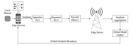
Figure 1.The training procedure of communication-efficient federated learning.

In this paper,we assume thatθis the parameter of global model trained at the edge server,Dkdenotes the local dataset of devicekand|Dk|denotes the size ofDk.The local loss function of devicekonθis as follows

which is the average of the sample-wise loss functionf(θ,xi,yi).f(θ,xi,yi) quantifeis the prediction deviation ofθon the training samplexiw.r.t its labelyi.The global loss function underθcan be given as

The training aims to fnid the minimum of global loss functionF(θ),and the minimum can be mathematically written as

To getθ*,the descent direction ofF(θ)is needed.SGD is proved to be effciient and well-behaved in large-scale dataset for searching the minimum of loss function,and then widely used in federated learning.In each iteration,for example,them-th iteration,each device uses the received global modelθ(m)to update the local loss function defnied in (1),and calculates the local stochastic gradient by using part of the local dataset.For devicek,the stochastic gradient offk(θ(m))can be calculated as

where∇denotes the derivation operation,is a part of local dataset of deviceskwith sizeb.

In practice,the local stochastic gradients consist of high-dimensional vectors or arrays,which even have millions of components.The limited battery capacity and wireless bandwidth of devices cannot satisfy the demand of fast transmitting these vectors/arrays.As a consequence,the communication bottleneck occurs,which calls for gradient compression before transmission.

Towards this regard,we frist sparsify each stochastic gradient and then quantize the remaining nonzero components by QSGD.This procedure is denoted as

whereTq(·) denotes the sparsifciation function in whichqbiggest components of a gradient are remained and transmitted while the rest are replaced by zero and neglected,andQs(·) is a quantization function with quantization levels.After receiving all the compressed local stochastic gradients,the edge server aggregates them to get the approximated global gradient as

whereηdenotes the learning rate (or step size).The updated global modelθ(m+1)is then broadcast to devices.The server-device iteration is completed until the global loss functionF(θ)is minimized.

III.PRELIMINARIES

In this section,we introduce some preliminaries used in our paper,including the concept of QSGD and Elias coding.

3.1 QSGD

In the quantization literature,the one-bit quantization and signSGD use 1 bit to quantize.Terngrad quantizes the positive,zero and negative components to +1,0 and -1,respectively.The above methods have fxied quantization degree.Thus,we select QSGD [16] as the quantization method in our scheme.It can adjust quantization degree by the adjustable parameter quantization levels.Furthermore,QSGD achieves a compromise between quantization variance and training accuracy.Some necessary concepts of QSGD is introduced as follows.

Let‖v‖2denote the L2 norm of vectorv,which is also the length of vectorv.For any scalarr ∈R,we letsgn(r)∈{-1,+1}whilesgn(0)=1,which means that the signs of the positive and negative scalars are+1 and-1,respectively.

QSGD belongs to scalar quantization,which quantizes the vector components to scalar codes respectively.Moreover,the codes are located uniformly in one-dimensional coordinate axis.An example is shown in Figure 2.We defnie a quantization functionQs(v),wheres ≥1 denotes the adjustable quantization level.In that case,the quantization interval is divided intos-1 uniform subintervals and endpoints of these subintervals are the codes.

Figure 2.An example of QSGD with s=5,where the point 0.6 is quantized to 0.5 with probility p and 0.75 with probility 1-p.

For any non-zero vectorv ∈Rn,Qs(v) is defnied as

whereviis thei-th component of vectorv,ξi(v,s)is an independent random variable which is the map ofand defnied as

wherejis an integer which makes sure that0≤j ＜s.p(a,s) is a probability function andp(a,s)=as-jfor anya ∈[0,1].The above quantization approach is unbiased and introduces minimal variance.That is,ξi(v,s) has minimal variance inThen,two properties of QSGD are given as follows

3.2 Elias Coding

In practice,stochastic gradient usually contains several high-dimensional arrays.We flatten these arrays,clip them to be vectors with the same lengthI,and useElias codingto encode the stochastic gradient after sparsifciation and quantization.

In QSGD,vectorv’s codeQs(v) can be expressed by tuple (‖v‖2,σ,ζ),whereσis a sign vector containing signs of all components ofv;ζis a vector and itsi-th component is an integer whose value iss·ξi(v,s).If the code of a vector can be accurately expressed by the tuple,the receiver can recover the initial vector after receiving the code.The so-called Elias coding method can encode this tuple[16].Given any tuple (‖v‖2,σ,ζ) with quantization levels,the coding method is described as follows.First,32 bits is used to encode‖v‖2.Next,it continues to encode the information ofσandζ.To begin with,the position of the frist non-zero entry ofζis encoded,and then a bit is appended to denote the sign of this entry,i.e.σi,followed byElias(s·ξi(v,s)).Iteratively,it proceeds to encode the distance of the next non-zero entry ofζto the current non-zero entry,then encode the nextσiands·ξi(v,s)in the same way.The decoding scheme is the inverse process of encoding: we frist read off the frist 32 bits to reconstruct‖v‖2,then use decoding method to read off the positions and values of the non-zero entries ofζandσiteratively.

IV.TOP-q BASED SPARSIFICATION

We adopt Top-qbased sparsifciation before QSGD.Note that Top-qsparsifciation is a well studied method.We do not focus the method itself but the transmission bits reduction under this method.Defnie the sparsifciation function asTq,in which we set a threshold such that only components larger than the threshold can go to the QSGD function.In Top-qsparsifciation,qcomponents with the largest absolute value are preserved.For a vectorv ∈RI,itsi-th component is defnied by

wherethris theq-th largest absolute value ofv’s components.

The transmission bits are related to the number of non-zero components of vectors and quantization levels.Assume that devicek’s local stochastic gradientgkhasPtuples(‖v‖2,σ,ζ)corresponding toPvectors.From Theorem 3.2 in reference[16],the number of transmission bits can be given as

We defnieβ ∈(0,1]as the fraction of the non-zero components after sparsifciation.That is

The reduction of communication overhead in bits w.r.t.sparsifciation factorβand quantization levelskis derived as follows

Theorem 1.For given β and sk,the reduction of communication overhead in bits are

where β denotes the percentage of the remaining components after sparsification,sk denotes quantization level of device k,I denotes the length of initial vectors,and P means that gradient gk has P vectors.

Proof.Please see Appendix A.

Next,we analyze the relationship about the overhead reductionBkversus the sparsifciation factorβand the quantization levelsk,respectively.Without loss of generality,we ignore the constant inBkand rewriteBkas

4.1 Bk Versus β

For givensk,we can obtain the following result aboutBkversusβ.

Proposition 1.There exit two quantization levels sk1and sk2,such that when sk ∈[1,sk1)or sk ∈[sk2,+∞),Bk decreases monotonically as β increases;when sk ∈[sk1,sk2),Bk first decreases and then increases monotonically as β increases.

Proof.Please see Appendix B

From Proposition 1,it observes that the quantization levelskaffects the relationship between communication overhead andβsignifciantly.In the range of[1,sk1]and[sk2,+∞),Bkis dominated byβand decreases as the growth ofβmonotonically.In[sk1,sk2],the effects ofβandskreach a compromise and thusBkhas an inflection point.We try to explain this phenomenon.It is intuitive that larger threshold(smallerβ)reduces more transmission bits.Whenskis small,βtakes the leading role and thusBkdecreases asβincreases.Then,larger quantization levelskneeds more transmission bits,which magnifeis the influence ofβ.As a result,larger quantization levelskmagnifeis the influence of compression and thus reduces more transmission bits.This opposite effect exactly offsets the impact ofβand is the reason of inflection point.Furthermore,as the growth ofβ,the influence of growingskbecomes limited andβtakes back the control.Bkdecreases monotonically as the growth ofβ.

4.2 Bk Versus sk

For any givensk3＞sk4andβ,we have

If we wantBk(β,sk3)-Bk(β,sk4)＞0,sk3andsk4should satisfy

Then we can obtain the following result aboutBkversusskas follows.

Proposition 2.For any given β,there always exits a quantization level sk5,such that when sk ∈[1,sk5),Bk decreases monotonically;when sk ∈(sk5,+∞),Bk increases monotonically.

Proposition 2 shows that the correlation betweenβandskstill exists.

V.CHANNEL-AWARE QUANTIZATION

To further compress the communication overhead,we need to choose the quantization level to quantize the remaining non-zero components after sparsifciation.

5.1 Learning Convergence Analysis

Based on the system model and the above preliminaries,we study the learning convergence rate of federated learning with communication compression.Before the analysis,we follow the stochastic optimization literature and give some general assumptions as in[20].

Assumption 1 (Lower Bound).For allθand a constantF*,we have that the global objective valueF(θ)≥F*.

Assumption 2 (Smoothness).For global objectiveF(θ),letdenote the gradient at pointθ=[θ1,θ2,···,θI]T.Then∀αandα=[α1,α2,···,αI]T,for some nonnegative constant vectorl=[l1,l2,···,lI]T,

Assumption 3 (Variance Bound).The stochastic gradientg(θ) is unbiased and it has coordinate bounded variance:whereσg=[σg1,σg2,···,σgI] is a constant vector with non-negative components.

Based on the above assumptions,we can get the following result.

Theorem 2.When sparsification and quantization are utilized in federated learning,the convergence result is

where M denotes the number of global iterations,denotes the square of the dynamic range of gradient vectors’components of device k,K denotes the number of participating devices,F(0)denotes the initial objective value,F*denotes the minimum of the objective defined in Assumption 1,l0=‖l‖∞with l defined in Assumption 2,β denotes the sparsification factor,sk denotes the quantization level of device k,η denotes the learning rate and I denotes the length of the stochastic gradient.

Proof.Please see Appendix C.

Through Theorem 2,we have several observations as follows.First,the increase of the number of global iterations (or communication rounds)Mleads to the convergence of federated learning.Second,to guarantee the convergence,the learning rateηshould satisfy the following conditions: a) due to feasibility,to make the convergence rate bounded,should be close to 1 as soon as possible.These requirements can be satisfeid during the training by adjusting the learning rateη,sparsifciation factorβand the gradient lengthI.Third,the more devices,the lower the upper bound.This is called multi-user gain.More participating devices can provide more local data for learning,and make the aggregated stochastic gradient closer to the central true gradient.

We note that the higher quantization precision,the better convergence performance.This result can be seen from Theorem 2.As the growth of quantization levelsk,the convergence upper bound decreases.This observation is in accordance with the fact that higher quantization level means less quantization loss and thus better training performance.We also prove the relationship between the convergence rate and sparsifciation factor.

Proposition 3.The convergence upper bound decreases monotonically as the sparsification factor β grows.

Proof.Please refer to Appendix D.

The conclusion is also expected,i.e.,largerβmeans more non-zero components are preserved after sparsifciation,so the edge server can obtain more data/information for training.

5.2 Quantization Resource Allocation

In this subsection,we propose a quantization level allocation scheme based on channel dynamics to improve the communication effciiency.To obtain more clear insights of quantization level on the training performance,we consider the given sparsifciation factorβand setβ=1 here.

Based on the discussion that more transmitted data/information can improve learning accuracy but cause heavier communication overhead,we optimize quantization levelskto strike the compromise between training behavior and communication bottleneck relief.From Theorem 2,it is observed that decreasing the upper bound(or improving the learning（accuracy）)is equivalent to minimize the term ofby ignoring the constants.

First,we simplify the form of the number of transmission bits afterElias codingin QSGD [16] under the practical assumptionI ≫sk:

wherecis a constant related to the dimension of the original vectorI.For devicek,transmission bits after coding should be no more than the bits transmitted at the transmission rate corresponding to its subchannel capacity during the same period.That is

whererkdenotes the Shannon capacity asrk=HereWandPindicate the bandwidth and the transmit power,respectively,hkdenotes the channel fading of devicek,andN0is the power of channel noise.

Then,we formulate the optimization problem of quantization resource allocation as follows

Constraint(22a)assures that the total transmission bits are under the channel capacity of MAC.If we relaxskto be a positive real number,the objective function becomes a convex function and the constraint is a convex set,so P1 becomes a convex optimization problem.The Lagrangian function is

whereγis the non-negative Lagrangian multiplier.According to the following KKT conditions

SinceL1(0)＜0 andL1(+∞)＞0,thenL1(sk)only has one null point,denoted assk7,in [1,+∞),which is the optimal solution of the Lagrangian function.Since this optimization problem belongs to convex problem,sk7is also the global optimum solution.sk7can be calculated by the bisection search method.This search has a computational complexity ofO(log(N)).

In addition,skshould be limited by devicek’s subchannel capacity.From(22b)along with(20),one can have the upper bound of each quantization level assk8:

VI.SIMULATION RESULTS

We consider a federated learning system with a single edge server andK=20 edge devices.The devices are uniformly distributed in the coverage of a base station (BS) which embeds the edge server.We assume channel noise is the Gaussian white noise.The simulation settings are given as follows:Our study includes two models on three datasets about image recognition tasks as [33].The frist model is a multilayerperceptron (MLP) with 2-hidden layers,which contains 200 units,respectively,and each unit uses ReLU activation.This MLP model is used for training on MNIST and Fashion-MNIST datasets.The second model is a CNN with two 5 × 5 convolution layers(the frist with 32 channels,the second with 64,each followed with a 2×2 max pooling layer),a fully connected layer with 512 units and ReLU activation,and a fnial softmax output layer.This CNN model is used for training on CIFAR-10 dataset.After training the classifeir model on training dataset,the classifeir will be evaluated by the testing dataset to prove its reliability.The test accuracy and training loss serve as metrics to verify the effciiency and reliability of the proposed scheme.

6.1 Performance Comparison

To evaluate the performance of the proposed scheme,we consider SGD and signSGD as benchmarks.All the schemes are in the same experimental settings and the power of the Gaussian white noise is -100 dBm.The curves of the test accuracy versus the number of global epochs(or communication rounds) and that of the training loss are shown in Figure 3.We can observe that SGD performs best,since there is no communication compression and thus the local gradients are transmitted to the server with the most reliability among the three schemes.Second,the proposed scheme achieves higher performance compared with the signSGD because of the higher quantization accuracy.

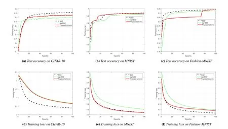
Figure 3.Performance comparison between different schemes.

6.2 Robustness to Noise

Note that the proposed scheme allocates the quantization levels based on channel dynamics of devices.To evaluate the robustness to channel noise,we investigate the performance of three schemes on MNIST dataset over different noise powers.In Figure 4 and Figure 5,we fnid that when noise power is small,all the schemes can maintain the training performance.However,when the noise power becomes larger,the performances of SGD and signSGD are degraded seriously while the proposed scheme still keeps the high test accuracy and low test loss.The reason for performance degradation of SGD and signSGD schemes is that their quantization levels are not adaptive to channel conditions,i.e.their quantization levels are constant during the whole training.The robustness to channel dynamics of the proposed scheme is proved.

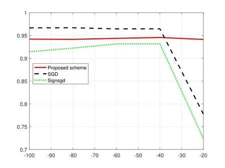
Figure 4.Accuracy comparison under different noise power.

Figure 5.Loss comparison under different noise power.

6.3 Overhead Reduction

We assume that the length of vectorIis 10000 and devicek’s local stochastic gradient hasP=6 arrays.Based on this,we investigate the relationship between the communication overhead reduction (bits)Bkand its two variables.The curve ofBkversusβis shown in Figure 6 and the curve ofBkversusskis shown in Figure 7.From Proposition 1 and Proposition 2,we fgiure out thatβandskhave complementary influences onBk.As forβ,Bkdecreases as it increases whenskis in the ranges of[1,sk1)and[sk2,+∞)while has an inflection point whenskbelongs to[sk1,sk2).Consideringsk,Bkalways decreases and then increases monotonically as the growth ofskno matter howβis valued.The above observations are in accordance with the theoretical analysis.

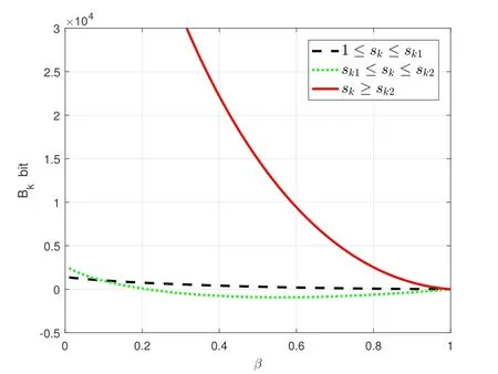
Figure 6.The relationship of Bk versus β.

Figure 7.The relationship Bk versus sk.

6.4 Adaptivity to Channel Condition

The curves of test accuracy and training loss under different channel capacities are shown in Figure 8.The larger channel capacity,the better training performance.The reason is that larger channel capacity allows devices to quantize stochastic gradients more precisely by using larger quantization levelsk.

Figure 8.Performance comparison under different channel capacities.

VII.CONCLUSION

In this paper,we focused on compressing communication overhead in federated learning over wireless networks by sparsifying and quantizing local stochastic gradients.Then,we analyzed the relationship of communication overhead reduction versus sparsifciation and quantization factors.The convergence rate of the proposed scheme was derived.Moreover,we proposed a quantization resource allocation scheme to enhance the learning performance.

ACKNOWLEDGEMENT

This paper was supported in part by the National Key Research and Development Program of China under Grant 2020YFB1807700 and in part by the National Science Foundation of China under Grant U200120122.

APPENDIX

A Proof of Theorem 1

After sparsifciation,the remaining components areβpercent of the initial vector’s components as shown in(13).Bringing(13)into(12),the transmission bits of thep-th vector after sparsifciation with quantization levelskis as follows:

Therefore,the reduction of the communication overhead is

According to the defniition in (9),we know thatξi(v,s)=0 ifQs(vi)=0.Then,

Until now we prove Theorem 1.

B Proof of Proposition 1

Then the value ofZis correlated withsk.We relaxskto real number and calculate the derivations ofZtosk,where there exist at least the frist and second derivations and they are both continuous:

C Proof of Theorem 2

Taking Assumption 2,we can get

Next,extending the expectation over randomness in the trajectory and performing a telescoping sum over all the iterations,we can get the lower bound ofF(0)-F*as

Rearranging(C.14),it follows that

Until now Theorem 2 is proved.

D Proof of Proposition 3

LetUdenote the convergence upper bound and make some rearrangement

Since 0＜β ＜1,we can know whetherU1is positive or not through the comparison betweenβ2and 1.Considering