SUN Guohao(孙国豪), YU Shui(余 水), FANG Xiu(方 秀), LU Jinhu(陆金虎)

School of Computer Science and Technology, Donghua University, Shanghai 201620, China

Abstract：Graph pattern matching (GPM) can be used to mine the key information in graphs. Exact GPM is one of the most commonly used methods among all the GPM-related methods, which aims to exactly find all subgraphs for a given query graph in a data graph. The exact GPM has been widely used in biological data analyses, social network analyses and other fields. In this paper, the applications of the exact GPM were first introduced, and the research progress of the exact GPM was summarized. Then, the related algorithms were introduced in detail, and the experiments on the state-of-the-art exact GPM algorithms were conducted to compare their performance. Based on the experimental results, the applicable scenarios of the algorithms were pointed out. New research opportunities in this area were proposed.

Key words：graph pattern matching (GPM); exact matching; subgraph isomorphism; graph embedding; subgraph matching

Introduction

In recent years, information and Internet technology have been developed rapidly, which leads to the era of big data. In this era, some common networks such as social networks[1-2], biological information networks[3-4]and communication networks[5-6]have produced massive amounts of heterogeneous data from multiple sources. With the increasing scale of data, the relationship among different data becomes more and more complex. The graph structure is very suitable to describe the internal correlation among multi-source heterogeneous data, which has been widely used in the fields of computer vision and pattern recognition[7-9].

Most networks can be modeled as graphs. How to analyze and mine the key information in a graph has become a research hotspot. Graph pattern matching (GPM) is a key technique for mining information in graphs, which aims to find out all isomorphic subgraphs of a given query graph in a data graph. GPM is also called subgraph isomorphism, which has been widely used in protein interaction network analyses[10-11], social network analyses[12-13], chemical compound searches[14], network intrusion detection[15-16], resource description framework (RDF) query processing[17-18], recommendation systems[19-20]and so on.

The GPM problem belongs to non-deterministic polynomial hard (NP-hard) problems[21-22], which makes it computationally expensive to find matching results, especially in large-scale graphs. In order to solve this problem, many efficient methods have been proposed both in static and dynamic graphs. Because of the difficulty of GPM in dynamic graphs, the research on dynamic graphs is still in its infancy[23]. The static GPM is focused on in this paper.

Based on the accuracy of the query results, the static GPM can be grouped into two categories: exact GPM and approximate GPM. The exact GPM requires that not only in labels and semantics but also in the structure, the vertices in a query graph and a data graph should be strictly matched. The approximate GPM relaxes the constraints of labels and semantics, which allows a label to match its subset labels and allows some errors in the matching results. In most practical applications, the matching results are often required to be accurate, which makes the exact GPM more widely used than the approximate GPM. Therefore, the exact GPM is focused on in this paper.

At present, many methods have been proposed in the field of the exact GPM. The most classic algorithm is Ullmann algorithm[24]. The Ullmann algorithm is a backtracking algorithm, which finds matching results by adding partial results. Based on the backtracking framework of the Ullmann algorithm, many efficient algorithms have been proposed to accelerate the exact GPM. The representative algorithms are VF2[25], GraphQL[26], GADDI[27], SPath[28], Turboiso[29], core-forest-leaf (CFL)[30], DPiso[31], compact embedding cluster index (CECI)[32]and RI[33].

In this paper, the applications and the research progress of the exact GPM are first summarized, and the related algorithms are introduced in detail. Then, the experiments on the latest exact GPM algorithms are conducted to compare their performance. Finally, the future research opportunities in this field are discussed.

1 Preliminaries

This paper focuses on the undirected vertex-labeled graphg=(V,E,W,L), whereV,EandWrepresent the vertex set, the edge set and the label set ofg, respectively;Lis a label function that maps a vertexuto a label. The notations frequently used in this paper are shown in Table 1.

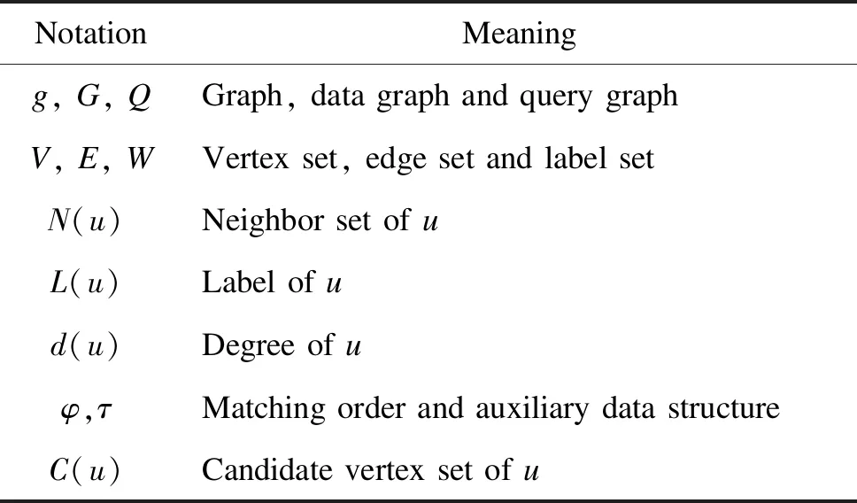
Table 1 Notations frequently used in this paper

Definition1Subgraph isomorphism: given a query graphQ=(VQ,EQ) and a data graphG=(VG,EG), a subgraph isomorphism is an injective functionffromVQtoVGsuch that ∀u∈VQ,L(u)=L(f(u)); ∀e(u,u′)∈EQ,e(f(u),f(u′))∈EG.

Definition2Label and degree filtering (LDF) constraint: given the query vertexu∈VQ, it can be matched to the data vertexv∈VGif the following conditions are satisfied:L(u)=L(v);d(u)≤d(v).

GivenQandG, the exact GPM aims to find in the data graph all the subgraphs that are the isomorphism of the query graph.

2 Exact GPM

2.1 Common framework

Leeetal.[34]proposed a common framework for some representative exact GPM algorithms. Sunetal.[35]supplemented this framework to make it suitable for more algorithms. The common framework is shown in Fig.1, which takesQandGas input and outputs all matching results fromQtoG.

Fig.1 Algorithm of common framework

2.2 Representative algorithms

The exact GPM algorithms can generally be divided into three steps. The exact GPM algorithms will use some pruning strategies or filtering methods to filter the candidate vertices in step 1. Step 1 is also called the filtering method of the exact GPM algorithms. The exact GPM algorithms will use some methods to generate a matching order in step 2. Step 2 is also called the ordering method of the exact GPM algorithms. The exact GPM algorithms will enumerate the matching results based on the filtered vertices and the generated matching order in step 3. Step 3 is also called the enumeration method of the exact GPM algorithms. This paper will introduce the representative exact GPM algorithms in detail according to the three steps.

2.2.1CFLalgorithm

Fig.2 Example of data and query graphs: (a) data graph G; (b) query graph Q

Fig.3 Example of filtering method of CFL: (a) BFS tree of query graph Q; (b) CPI structure of query graph Q

Step2The ordering method of the CFL algorithm uses a path-based strategy for generating the matching order. Specifically, this method first selects three vertices from the core structure with a higher degree and a lower frequency of labels in the data graph label set and chooses the vertex with the smallest candidate vertices as the first vertex in the matching order. Then, this method constructs a weight array to count the embeddings of all paths from the root to leaves in the BFS tree of the query graph in the CPI structure. LetC(p) represent the embeddings of the pathp, andNTE(p) represent the number of edges connected with the vertices in the pathpin the query graph. This method selects the pathp*with the minimum value ofC(p)/|NTE(p)|, and adds the vertices in the pathp*to the matching order. It removes the pathp*. Setu+as the last vertex of the common prefix of the pathpand the matching order sequence.pu+is the suffix ofpstarting fromu+. This method selects the pathp*with the minimum value ofC(pu+)/|C(u+)|, and adds the vertices that in the pathp*but not in the current matching order into the matching order. Then, this method removes the pathp*until all paths are processed and a matching order is generated.

Step3The enumeration method of the CFL algorithm matches each query vertex to its candidates with the matching order based on the backtracking method, which is the same as the Ullmann algorithm.

The efficiency of the CFL algorithm is much higher than that of the previous algorithms such as Turboiso, GraphQL and SPath.

2.2.2DPisoalgorithm

The CPI structure of the CFL algorithm is generated according to the BFS tree of the query graph. However, the BFS tree cannot contain all the edges in the query graph, and the non-tree edges (e.g., the edges not in the BFS tree) have a strong pruning ability.

Step1The filtering method of the DPisoalgorithm reconstructs the query graph into a directed acyclic graph (DAG) and designs a auxiliary data structure called the candidate space (CS) structure. The CS structure can replace the data graph for the matching query process. Figure 4(a) shows the DAG of the query graphQin Fig.2(b), and Fig.4(b) shows its CS structure.

Fig.4 Example of filtering method of DPiso: (a) DAG of query graph Q; (b) CS structure of query graph Q

The filtering method of the DPisoalgorithm applies the same method as the CFL algorithm to generate candidate vertex sets according to the CS structure. This method also needs to satisfy LDF and NLF constraints. For anyv∈C(u), letpt(u) represent the prefix tree ofu, which consists of the path starting fromuto all leaf vertices. If the prefix treept(u) can be homomorphic mapped to the prefix treept(v) (i.e., all the vertices inpt(u) can be matched to the vertices inpt(v) and allow duplicate matching of vertices), thenvcan be kept inC(u).

Step2The ordering method of the DPisoalgorithm separates all the vertices of which degree is one in the query graphQ, and the remaining vertices are recorded asQ′. The ordering method of the DPisoalgorithm matches the vertices inQ′. This method selects the vertex with the smallest number ofω(u), andω(u) is an estimate of the path embeddings. Foru∈V(Q′), this method constructs the tree-like path ofu. A tree-like path starting fromuindicates that the vertices have only one parent vertex apart from the first vertex. Let the embeddings of the tree-like path ofuin the CS structure be denoted asω(u), and for eachu∈V(Q′), this method constructs the weight array according toω(u), where the vertex with the least weight is selected as the next matching vertex. Moreover, an optimization method called failing set pruning strategy is also proposed by the DPisoalgorithm, which applies the relevant information to exclude some useless vertices in the search tree of the partial matching.

An example of the failing set pruning strategy is shown in Fig.5. Figure 5(c) shows the process of the failing set pruning strategy ofQinG. The vertices in the tree represent a partial matching resultM.(ui,vj) means thatuican be matched tovj, and !(ui,vj) means thatuicannot be matched tovj. When matchingu3tou10after matchingu4tov11, it will fail in the end. The reason is that there is no isomorphic subgraph in the data graph that can be matched to the query graph. Therefore, the failing set pruning strategy removes all the sibling vertices (M3,2,M3,3, …,M3,10) of the search vertexM3,1. In other words, there is no need to matchu4to other vertices.

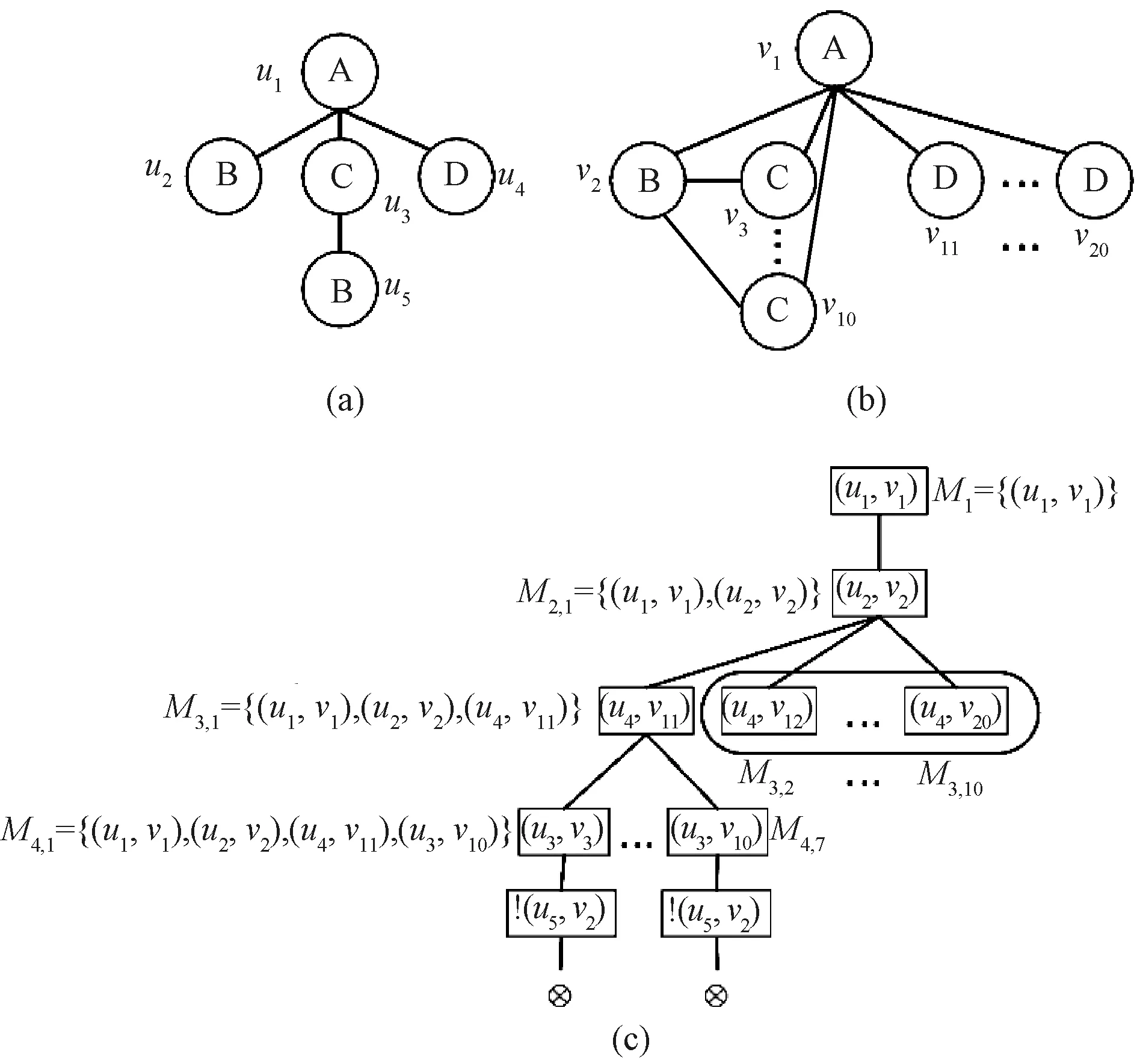
Fig.5 Example of failing set pruning strategy: (a) query graph Q; (b) data graph G; (c) search tree of Q in G

Step3The enumeration method of the DPisoalgorithm enumerates the matching result with the matching order, which is the same as the Ullmann algorithm.

The DPisoalgorithm is much more efficient than the CFL algorithm.

2.2.3CECIalgorithm

Step2The ordering method of the CECI algorithm first selects a vertex with a larger degree and a smaller number of initial candidates as the first vertex in the matching order. Then, it conducts the breadth-first search from this vertex, and the order of the width-first search is taken as the matching order.

Step3The enumeration method of the CECI algorithm enumerates the matching result with the matching order, which is the same as the Ullmann algorithm.

The CECI algorithm is more efficient in the parallel processing field.

2.2.4RIalgorithm

The core idea of the RI algorithm is to find an efficient matching order as a good matching order is very important to speed up the matching process.

Step1The filtering method of the RI algorithm filters the candidate vertices based on two pruning rules of the Ullmann algorithm.

(1) One to one mapping relationship. For example, the subgraph matching procedure ofQinGwith matching orderφ={u1,u2,u3} is shown in Fig.6. In Fig.6(c),u1is adjacent tou2, andv1is not adjacent tov5. Ifu1is matched tov1, then there is no need to matchu2tov5.

Fig.6 Example of subgraph matching procedure: (a) query graph Q; (b) data graph G; (c) search tree of Q in G

(2) The consistency of adjacent relations of vertices. For example, a query vertex can only match one data vertex.

Step2The ordering method of the RI algorithm applies a score function to calculate the score of a vertex according to the topological structure information of the query graph. Specifically, this method first selects a vertex with the largest degree in the query graph as the first vertex in the matching order. LetV1represent the set of neighbors ofu∈V(Q) that are in the current matching orderφ,V1={u′∈φ|e(u,u′)∈E(Q)}. LetV2that is not inφrepresent the set of common neighbors betweenuand the vertices inφ,V2={u′'∈φ|∃u″∈V(Q)-φ,e(u′,u″)∈E(Q)∧e(u,u″)∈E(Q)}. LetV3represent the set of neighbors ofuthat are not inφand not adjacent to any vertices inφ,V3={u′∈N(u)-φ|∀u″∈φ,e(u′,u″)∉E(Q)}.

This method iteratively selects the vertex with the largest |V1| as the next vertex. If |V1| is the same, the vertex with the largest |V2| is selected. If |V1| and |V2| are the same, the vertex with the largest |V3| is selected. If all three are the same, the vertex is selected at random.

Step3The enumeration method of the RI algorithm enumerates the matching result to the matching order, which is the same as the Ullmann algorithm.

Compared with the latest algorithms, the matching order of the RI algorithm is very efficient. The RI algorithm is only suitable for small queries because it does not use any data graph information.

3 Experiments

In this section, the latest exact GPM algorithms for experiments are compared, which are CFL, DPiso, CECI and RI algorithms.

3.1 Experiment environment

The experiments are conducted on a Linux machine with the Ubuntu 20.04.1 64 bit distribution operating system. The processor model is AMD ryzen 5 4600H 3.00 GHz and the memory is 8 G. All the algorithms are programmed in C++.

3.2 Datasets and query graph

Yeast, Human Protein Reference Database (HPRD), WordNet and Youtube datasets are selected in this experiments, which are commonly used in the previous work. The details of these datasets are shown in Table 2, wheredmaxrepresents the maximum degree of vertices,Wmaxrepresents the maximum frequency of labels, andddenotes the average degree of vertices. |V|, |E| and |W| represent the number of the vertices, the number of the edges and the number of the labels, respectively. The query graphs are generated for each datasetGby randomly extracting subgraphs fromG, and each query graph can be guaranteed to have at least one matching result in this way. For each dataset, five query sets are generated according to the number of vertices. The number of vertices are used to measure the scale of the query graph.

Table 2 Properties of datasets

3.3 Experimental results and analysis

The size of the query graph is measured by the number of vertices. For example, a query graph size of four means that it contains four vertices. For Yeast and HPRD datasets, the query graphs are varied with sizes of 4, 8, 16, 24 and 32. For WordNet dataset, the query graphs are varied with sizes of 4, 8, 12 and 16, because WordNet dataset contains a large number of the same labels, which makes it very challenging.

3.3.1Efficiency

Figure 7 shows the average elapsed time of the exact GPM algorithms by varying the query graph size.

Fig.7 Average elapsed time of algorithms by varying query graph size: (a) Yeast dataset; (b) HPRD dataset; (c) WordNet dataset; (d) Youtube dataset

On Yeast dataset, the overall performance of the CECI algorithm is the best. The overall efficiency of the DPisoalgorithm is very close to that of the CECI algorithm. The RI algorithm has the worst efficiency. On HPRD dataset, the overall performance of the CFL algorithm is the best. On WordNet dataset, when the query graph size is 16, the overall performance of the RI algorithm is the best, and the CFL algorithm is the worst among all the algorithms. On Youtube dataset, the performance of the CFL algorithm is the worst and the RI algorithm is the best when the query graph size is 16.

On Yeast dataset, when the query graph is dense, the DPisoalgorithm and the CECI algorithm conduct one more refinement on the candidate vertex set than the CFL algorithm, and the DPisoalgorithm and the CECI algorithm are better than the CFL algorithm. Moreover, the DPisoalgorithm and the CECI algorithm both apply the set intersection-based method for further filters, which speeds up the matching process. The RI algorithm is faster than the CFL algorithm, the DPisoalgorithm and the CECI algorithm when the query graph size is four, because the purpose of the RI algorithm is to find the best matching order to speed up the matching process and there are no efficient pruning rules or reasonable auxiliary data structures. The performance of the RI algorithm is relatively good when the dataset is sparse. Experiments on HPRD dataset show that all queries can be completed in 10 ms on average, so it is relatively easy to query on HPRD dataset. The DPisoalgorithm conducts one more refinement on the candidate vertex set than the CFL algorithm, so it is slower than the CFL algorithm in this dataset. The extra refinement process does not achieve good efficiency because it is easy to query on this dataset, which increases the time cost. In addition, the failing set pruning strategy of the DPisoalgorithm is effective on large queries. On WordNet and Youtube datasets, the overall performance of the DPisoalgorithm and that of the CECI algorithm are similar, and both of them are superior to the CFL algorithm. It is because the WordNet dataset contains a large number of duplicate labels and the average degree is only 3.1, which makes the dataset sparse. The overall performance of the RI algorithm is better than that of other three algorithms in the sparse graphs. In summary, the performance of the DPisoalgorithm and the CECI algorithm is better than that of the CFL algorithm and the RI algorithm. The matching performance of the CECI algorithm and that of the DPisoalgorithm is close.

In addition, the experimental results also demonstrate that the characteristics of both pattern graphs and data graphs will influence the efficiency of the algorithms. On WordNet dataset, the RI algorithm is better than other three algorithms in the sparse graphs. For the dense pattern graph, the DPisoalgorithm and the CECI algorithm can achieve better efficiency because they conduct one more refinement on the candidate vertex set. Therefore, based on the results, when facing a new pattern graph and a new data graph, we can first analyze the characteristics of both the pattern graph and the data graph, and then select the suitable algorithm in order to achieve the best efficiency when performing the exact GPM progress.

3.3.2Memorycost

Figure 8 shows the average memory cost of the exact matching algorithms by varying the query graph size. The memory cost of the RI algorithm is the largest among all algorithms on Yeast, HPRD and Youtube datasets.

The RI algorithm does not build any auxiliary structures to help filter vertices, and its filtering method is inefficient compared to other algorithms. Therefore, it consumes too much memory.

In summary, the RI algorithm consumes more memory than other algorithms on Yeast, HPRD and Youtube datasets, and the overall memory cost of CFL, DPisoand CECI algorithms is similar. On WordNet dataset, the average memory cost of the CECI algorithm is significantly less than that of the CFL algorithm and the DPisoalgorithm.

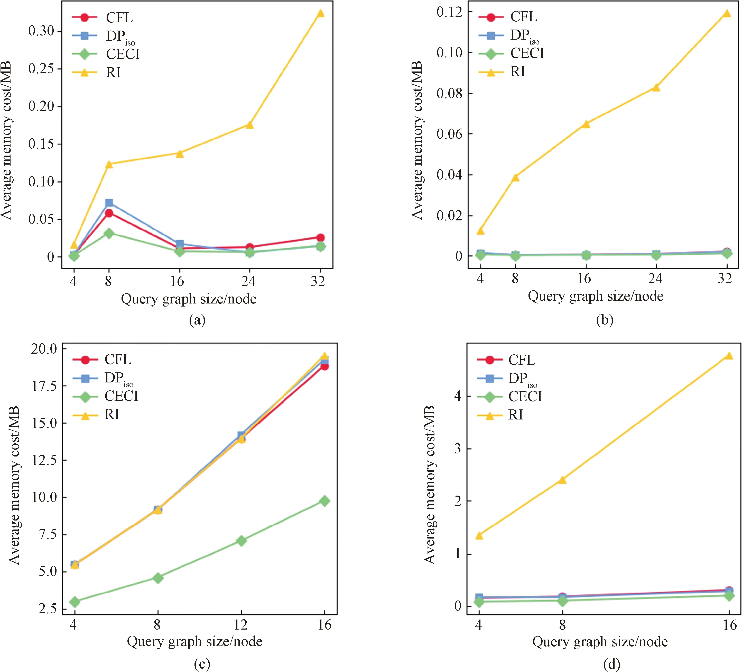
Fig.8 Average memory cost of algorithms by varying query graph size: (a) Yeast dataset; (b) HPRD dataset; (c) WordNet dataset; (d) Youtube dataset

4 Conclusions

In this paper, the applications of the GPM technique were introduced. Then, the typical GPM algorithms were presented in detail and the performance of these algorithms was compared. The efficiency in the different data graphs and query graphs of algorithms was shown, which could help us to select appropriate algorithms in different scenarios to achieve high query efficiency.

In the future, we can conduct the exact GPM in a distributed environment to improve the performance,i.e., divide the large-scale data graph into multiple parts, process each part in parallel in different computer memories, and finally summarize the processing results of all machines into a complete result. It is also a good future research direction for the development of distributed GPM algorithms because they can handle highly dynamic data graphs. In order to reduce the size of the data graph, it is also an interesting future work to develop a general graph compression technique that maintains the matching properties of subgraphs in a distributed environment. Since most of the current exact GPMs are for the static graphs, the data graph is constantly updated in actual scenarios. Therefore, it is important to design efficient dynamic graph matching algorithms. Moreover, some of the latest documents have begun to optimize GPM from the computer hardware level to speed up the matching speed, such as using field programmable gate array to accelerate the subgraph matching process on a single computer, and using single instruction multiple data instructions to enhance pruning capabilities. Therefore, optimizing GPM from the hardware level will be an interesting job.