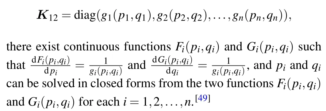
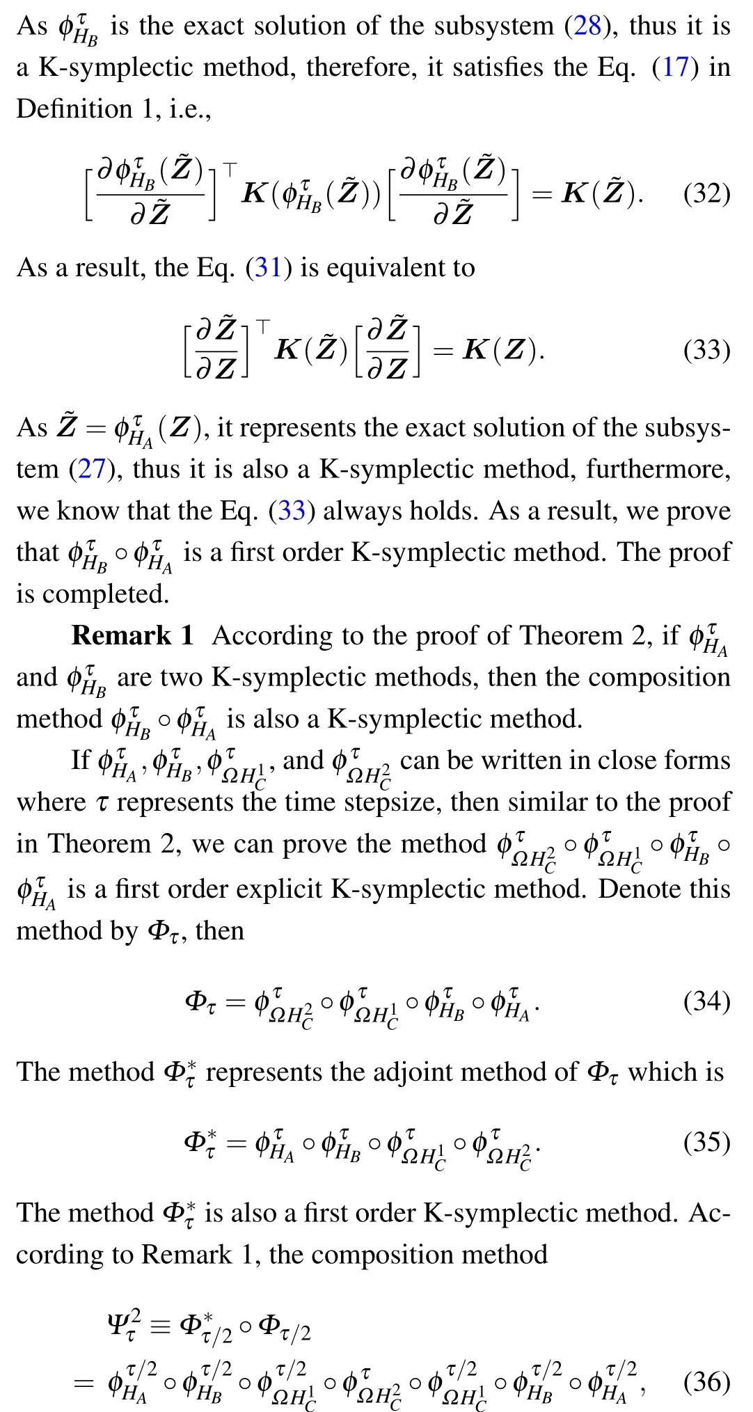
Explicit K-symplectic methods for nonseparable non-canonical Hamiltonian systems
2023-03-13BeibeiZhu朱贝贝LunJi纪伦AiqingZhu祝爱卿andYifaTang唐贻发
Beibei Zhu(朱贝贝) Lun Ji(纪伦) Aiqing Zhu(祝爱卿) and Yifa Tang(唐贻发)
1School of Mathematics and Physics,University of Science and Technology Beijing,Beijing 100083,China
2LSEC,ICMSEC,Academy of Mathematics and Systems Science,Chinese Academy of Sciences,Beijing 100190,China
3School of Mathematical Sciences,University of Chinese Academy of Sciences,Beijing 100049,China
Keywords: non-canonical Hamiltonian systems, nonseparable, explicit K-symplectic methods, splitting method
1.Introduction
Many mechanical systems can be expressed as noncanonical Hamiltonian systems, such as the Lotka-Volterra model,[1]the nonlinear Schr¨odinger equation,[2-5]the charged particle system,[6,7]the guiding center system,[8-10]the Maxwell-Vlasov equations[11,12]and the ideal MHD formualtion.[13]These models appear in many applications of areas.The Lotka-Volterra model[1]is the simplest model of predator-prey interactions and it describes the growth of animal species.It was first established in mathematical biology, then it had been derived independently in the fields of epidemics, combustion theory and economics, and other disciplines.The nonlinear Schr¨odinger equation[2-5]is a very important completely integrable model in soliton theory.It appears in many physical areas, such as nonlinear optics,plasma physics, and bimolecular dynamics.The motion of charged particles[6,7]in external electromagnetic fields is the most fundamental equation in plasma physics research.It contains the fast gyromotion and the slow gyrocenter motion.If we average out the fast gyromotion from the charged particle motion, the motion of the gyrocenter is obtained.The non-canonical Hamiltonian systems are generalizations of the canonical Hamiltonian systems.[1,14-18]They have noncanonical symplectic structures which are preserved by the K-symplectic methods.K-symplectic methods exhibit advantageous energy preservation properties just like the symplectic methods[3,19-23]for Hamiltonian systems.Therefore, Ksymplectic methods are preferred methods for long time simulations of non-canonical Hamiltonian systems.One approach to constructing K-symplectic methods for a non-canonical system is to transform the system to a canonical one by a coordinate transformtion[1,14]and use the symplectic method.The other approach is the generating function method,[15,24]but it is also inevitable to seek for one coordinate transformation.To avoid the difficulty of finding the coordinate transformation,we prefer to use the splitting method for the non-canonical Hamiltonian systems.
Symplectic methods exhibit superior long-term behavior compared with standard integrators such as explicit Runge-Kutta methods.The long-term behaviors include the slower error growth and the approximate preservation of invariants,such as the energy and the angular momentum,without secular drift.Symplectic methods can be classified as the explicit ones and the implicit ones.If the Hamiltonian can be separated into several integrable parts, then explicit symplectic methods can be constructed by composing the analytical solutions of the sub-Hamiltonians.The typical examples of explicit symplectic methods are the second-order leapfrog method,[25]the fourth-order Forest-Ruth method,[26]and the Yoshida’s fourth-order method.[23]For nonseparable Hamiltonian systems, implicit symplectic methods are always available.Implicit symplectic methods have completely implicit symplectic methods including the implicit midpoint rule,[27,28]the implicit Gauss-Legendre Runge-Kutta symplectic method,[29,30]and the explicit and implicit mixed symplectic methods.[31-34]The implicit methods are numerically more expensive than the explicit methods because one of the iteration methods is required to solve the equations.On the other hand,the implicit methods perform better in solving stiff equations than that of the explicit ones.[35]
Recently, a fourth order non-canonical explicit and implicit symplectic integrator for post-Newtonian(PN)Hamiltonian of spinning compact binaries was constructed by splitting the Hamiltonian to orbital and spin contributions and the integrator exhibited excellent long-term performance.[31]Using the canonical spin variables suggested in Ref.[36],some canonical symplectic methods for PN Hamiltonian of spinning compact binaries were obtained.[32-34]By splitting the Hamiltonian into separable and nonseparable parts,Zhonget al.developed the fourth-order explicit and implicit mixed symplectic integrators.[32]The explicit leapfrog method was used to calculate the separable Hamiltonians while the implicit midpoint rule was used to solve the nonseparable Hamiltonians.[32]Meiet al.discussed the numerical performances of the Forest-Ruth symplectic method and the Yoshida symplectic method by several examples including the PN Hamiltonian formulation of non-spin compact binaries.[33]For the 10-dimensional PN canonical conservative Hamiltonian system,Meiet al.explored the influences of the spin effects of black hole pairs on the dynamics and showed that the chaos occurs when the spin-spin effects of the two spinning bodies were included by combining the numerical tests.[34]In fact, when the dissipative forceFis set to zero, the noncanonical post-Newtonian Hamiltonian of spinning compact binaries takes the form
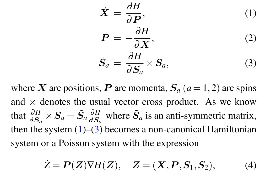
whereP(Z)is an anti-symmetric matrix and satisfies the Jacobi identity which is defined below in Eq.(10).Poisson systems are generalized non-canonical Hamiltonian systems.The matrixP(Z) in Poisson systems can be singular.When the matrixP(Z)is nonsingular,the Poisson system becomes the non-canonical Hamiltonian system.
A class of explicit symplectic integrators based on operator splitting and composing have been developed recently for nonseparable systems, such as the charged particles around Schwarzschild black holes,[25,37-39]Reissner-Nordstr¨om black holes,[40-42]and Kerr black holes.[43-45]By splitting the Hamiltonian of Schwarzschild spacetime geometry into four integrable parts whose analytical solutions can be expressed as explicit functions,second order and fourth order explicit symplectic integrators were constructed.[25]The same technique was also used to construct explicit symplectic integrators for charged particles moving around a Reissner-Nordstr¨om black hole with an external magnetic field[40]and Reissner-Nordstr¨om-(anti)-de Sitter black hole with an external magnetic field.[41]Second order and fourth order explicit symplectic integrators were proposed for the Kerr spacetime geometry by using a time transformation function to obtain a transformed Hamiltonian where the operator splitting and composing can be directly used.[45]Following the work of Wuet al.,[45]explicit symplectic integrators were applied to study chaos of charged particles around the magnetized Kerr black hole.[43]How the small changes of parameters effect the dynamics of charged particles around the Kerr black holes immersed in an external magnetic field were also investigated.[44]Furthermore, by using the technique of the time-transformed explicit symplectic integrators for the Kerr-type spacetimes introduced in Ref.[45], Zhanget al.proposed explicit symplectic integrators for the deformed Schwarzschild black hole immersed in an external magnetic field and the obtained integrators exhibited good long-term performance for both regular orbits and chaotic orbits.[38]All the explicit symplectic integrators constructed above are applied to the canonical Hamiltonian system
where the symplectic matrixJis defined in Eq.(11).If the HamiltonianHcan be separated into two partsH(Z)=H1(Z)+H2(Z) withZ=(P,Q)∈R2n, we can define two differential operators
If the two sub-Hamiltonians have analytical solutions which can be expressed as explicit functions,then the composing integrator exphBexphA(Z0)is a first order explicit symplectic integrator.Higher order explicit symplectic integrators can be constructed by composing exphBand exphA.This operator splitting and composing technique can also be applied to the non-canonical Hamiltonian system (4) with nonsingularP(Z), but the differential operators are defined in a different way.Assuming that we split the HamiltonianHintoH(Z) =H1(Z)+H2(Z), the two differential operatorsD1andD2acting on a functionFare defined as follows:
With the above two operators, if the two sub-Hamiltonians have explicit analytical solutions, then we know that the integrator exphD2exphD1(Z0) is a first order explicit Ksymplectic integrator.Higher order explicit K-symplectic integrators can also be constructed by using composing technique.
The splitting method is widely used to construct explicit symplectic methods for separable Hamiltonian systems[1,46,47]and explicit K-symplectic methods for non-canonical Hamiltonian systems.[6,48,49]Blanes and Moan used the splitting method to construct an efficient fourth order symplectic method for non-autonomous Hamiltonian systems.[46]Heet al.used the splitting method[6]to construct the explicit Ksympletic methods for the non-canonical charged particle system.Zhuet al.constructed the explicit K-symplectic methods for both the bright solitons motion and the dark solitons motion of the nonlinear Schr¨odinger equation.[48,49]The explicit symplectic methods and K-symplectic methods had been constructed for separable systems while the work is much less for the nonseparable systems.For several subclasses of nonseparable Hamiltonian systems,Pihajoki constructed the explicit extended phase space symplectic-like methods based on the idea of extending the phase space by making two copies of it and using the splitting method.[50]These methods have good long-term performance in preserving the energy but are not symplectic both in the original phase space and the extended phase space because they are combined with coordinate mixing transformations.Inspired by the Pihajoki’s work, several researchers developed the phase space mixing maps.[51,52]Liuet al.compared several mixing maps and showed that the leapfrog method with the sequent permutations of coordinates and momenta can provide the most accurate results and the best long-term stable error behaviour.[51]A fourth order extended phase space explicit symplectic-like method with the sequent permutations of coordinates and momenta were proposed to solve four-dimensional metric of relativistic coreshell models with nonseparable Hamiltonian and the dynamics of chaos of the system was investigated.[53]Then, the midpoint permutation map was proposed and proved to have better performance.Luoet al.developed the midpoint permutation map for the fourth-order Yoshida’s method and showed that the midpoint permutation is more powerful in restraining the original phase space and the copying ones than that of the sequent permutations of coordinates and momenta.[52]Liet al.developed three fourth order explicit symplectic-like integrators by combining the extended phase space with the midpoint permutation and the sequent permutations of coordinates and momenta and got the same conclusion as Luoet al.that the midpoint permutation has the best performance.[54]The Yoshida’s fourth order extended phase space symplecticlike method with the midpoint permutation was applied to the problem of neutral particles around a Schwarzschild black hole and the dynamics of generic orbits by using this numerical method was surveyed.[55]Panet al.also applied the Yoshida’s fourth order extended phase space symplectic-like method with the midpoint permutation to solve the coherent post-Newtonian Euler-Lagrange equations and showed that the method behaves well in energy and/or angular momentum conservation over long time.[56]To overcome the short-term simulation problem of the Pihajoki’s work,Tao imposed a mechanical restraint with a control parameterΩon the two copies of the phase space and successfully realized the long-term simulation.[57]The recent literature pointed out that there is no universal method that can find the best choice of the control parameter in the Tao’s methods.[26]On the other hand,it was shown that the fourth order symplectic Yoshida’s method and Suziki-like method which are constructed based on the Tao’s idea were inferior to the fourth order nonsymplectic symmetric Forest-Ruth-like method with the midpoint permutation.[26]The Tao’s methods were also shown not superior to the extended phase space symplectic-like methods with the midpoint permutation proposed by Luoet al.[52]at the same order in accuracy.[39]Recently,semi-explicit symplectic integrators for nonseparable Hamiltonian systems, which are symplectic in both the original phase space and the extended phase space, were proposed.[58,59]These methods have good longterm performance in preserving the invariants and exhibit the same and even better efficiency than that of the Tao’s method.All the articles mentioned above construct symplectic methods or symplectic-like methods for nonseparable Hamiltonian systems.Different from them,we concentrate on the nonseparable non-canonical Hamiltonian systems.Our work is based on the pioneer work of Pihajoki and Tao,we construct the explicit K-symplectic methods for nonseparable non-canonical Hamiltonian systems by using the splitting method.As the non-canonical systems are more complicate than the canonical systems, in some cases the two copies of the phase space are not enough to construct explicit K-symplectic methods, thus we need to make more copies.
Nonseparable systems are important gradients of non-canonical Hamiltonian systems.The guiding center system,[8-10]the reduced magnetohydrodynamics equations,[60]and the Ablowitz-Ladik model of the nonlinear Schr¨odinger equation under periodic condition[1]are all nonseparable non-canonical Hamiltonian systems.Thus, it is critical to construct K-symplectic methods with long-term conservation property for nonseparable non-canonical systems.The idea is to extend the phase space and make several copies of the phase space and to impose an artificial restraint for the several copies of the phase space.The extended phase space Hamiltonian consists of several copies of the original Hamiltonian and another HamiltonianHcwith control parameterΩthat are used to control the copies of the variables.The constructed method is explicit and K-symplectic in the extended phase space.We extend the non-canonical systems in two ways according to their structures and analyze in which situation that the explicit K-symplectic methods can be constructed.Then we propose a second-order and a fourth-order explicit methods which are K-symplectic in the extend phase space but not K-symplectic in the original phase space.In order to characterize the distance between the new Hamiltonian ˆHwhich is exactly preserved by ap-th order K-symplectic method and the extended phase space Hamiltonian ¯H, we provide an error analysis on the Hamiltonian.The error analysis shows that the ˆHprovides an approximation to ¯H.To show the superiority of the K-symplectic methods in structure preservation and efficiency,we compare them with higher order explicit Runge-Kutta methods,[61,62]the implicit symplectic methods,the explicit and implicit symplectic methods for the original nonseparable noncanonical Hamiltonians,several other fourth order explicit K-symplectic methods for the extended phase space Hamiltonians, and several fourth order extended phase space K-symplectic-like methods with the midpoint permutation.
The paper is organized as follows.Section 2 is focus on constructing K-symplectic methods for the nonseparable systems with special structure and analyzing the situation in which the explicit K-symplectic methods can be constructed.In Section 3, the nonseparable systems are general systems and we make several copies of the phase space in order to construct explicit K-symplectic methods.Section 4 provides an error analysis from the view of Hamiltonian.In Section 5,all the numerical methods are listed and the numerical results in two nonseparable systems are provided.Finally,we give a short conclusion in Section 6.
2.Explicit K-symplectic methods for nonseparable systems with special structure
Consider the non-canonical Hamiltonian system
where the dot·represents the derivative with respect to timetand the functionHis the Hamiltonian.The matrixK=(lij)2n×2nis anti-symmetric, i.e.,li j=-lji.It is nonsingular,i.e.,detK(Z)/=0.Meanwhile,it satisfies the Jacobi identity
If we replace the matrixK-1(Z) with the constant matrixJ-1where
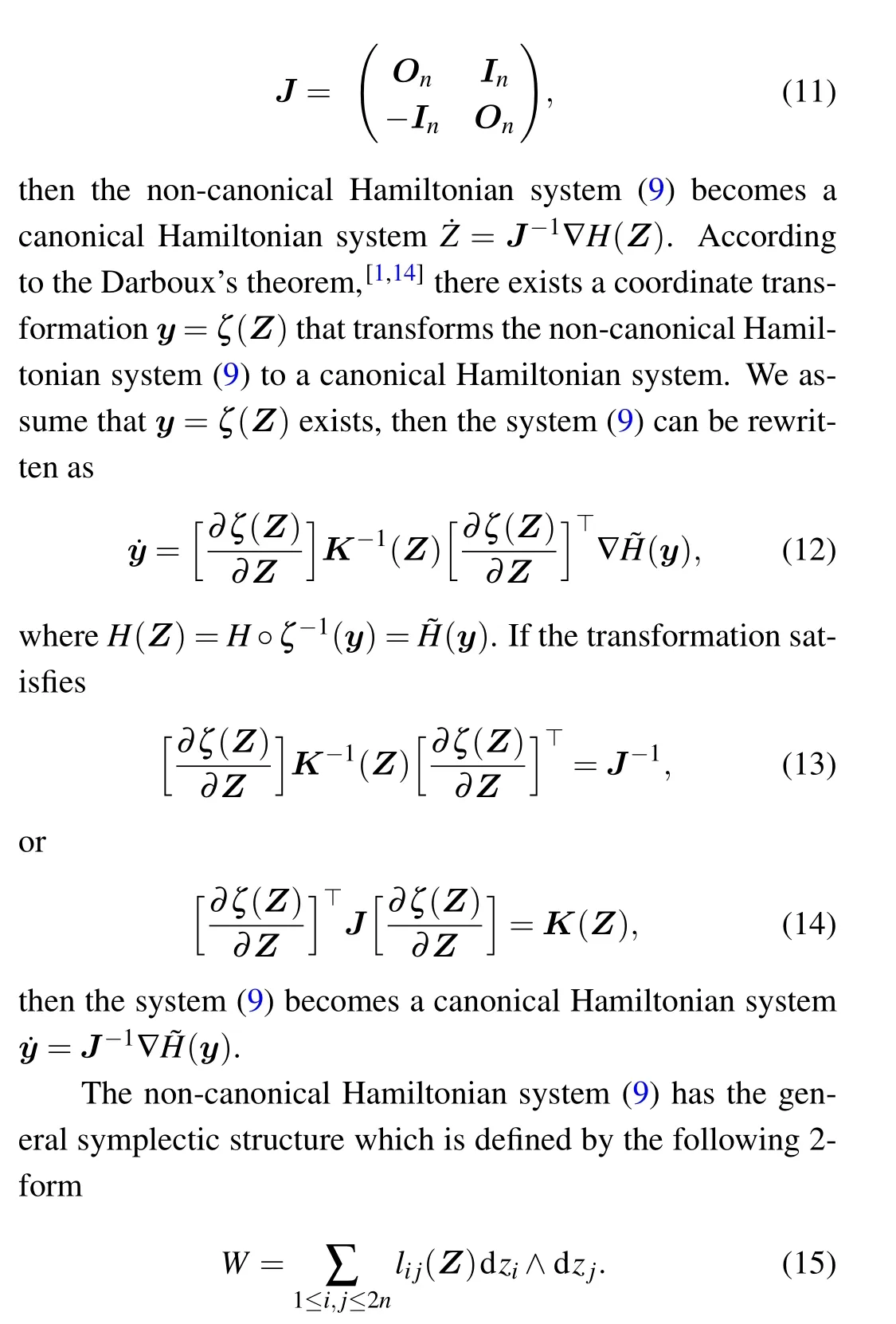
The above 2-form[14]is closed,i.e.,dW=0.The general symplectic structure is also called K-symplectic structure which is related to the matrixK(Z).The exact phase flow(exact solution)φt(Z) of the non-canonical Hamiltonian system is usually difficult to solve.However,we can use numerical methods that exactly preserve the K-symplectic structure of the noncanonical system.This kind of numerical methods is called K-symplectic methods.It is well known that the exact flowφt(Z)is one of the K-symplectic methods.On the other hand,the Hamiltonian is exactly preserved by the exact phase flowφt(Z),i.e.,
the last equality holds becauseK-1is an anti-symmetric matrix.ThusH(φt(Z))=H(φ0(Z))=H(Z0).Now we give the definition of the K-symplectic methods.
Definition 1 Given a numerical methodGτ:Z →ˆZ,if its Jacobian satisfies
we call it as a K-symplectic method.[1]
It is a difficult task to construct the K-symplectic methods for the general non-canonical Hamiltonian systems.[1]However,we can construct the K-symplectic methods for the separable non-canonical Hamiltonian systems by using the splitting method in some cases.The problem is whether we can use the splitting method to construct the K-symplectic methods for the nonseparable non-canonical Hamiltonian systems.
Here the form of the matrixK-1is assumed as
whereOnis then×nzero matrix.We approximate the flow of the non-canonical Hamiltonian system with an arbitrary nonseparableH(P,Q).The Hamiltonian is called separable ifH(P,Q)=H1(P)+H2(Q).[1]If the Hamiltonian does not satisfy the above form,it is called nonseparable.
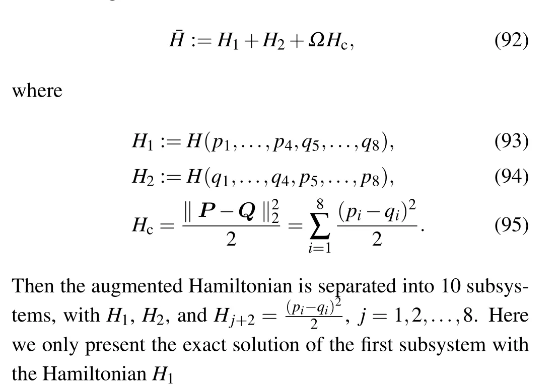
We aim at constructing higher order explicit K-symplectic methods of the system(9)with nonseparableHby considering an augmented Hamiltonian[57]

The original initial value problem is
and the extended system is
It should be noted that ifp(t) =x(t) in the extended system (22), then the extended system is just the two copies of the original system, thus we have the same exact solutionp(t)=x(t)=P(t),q(t)=y(t)=Q(t) if the same initial values are imposed onp,x,Pandq,y,Q.
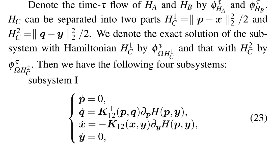
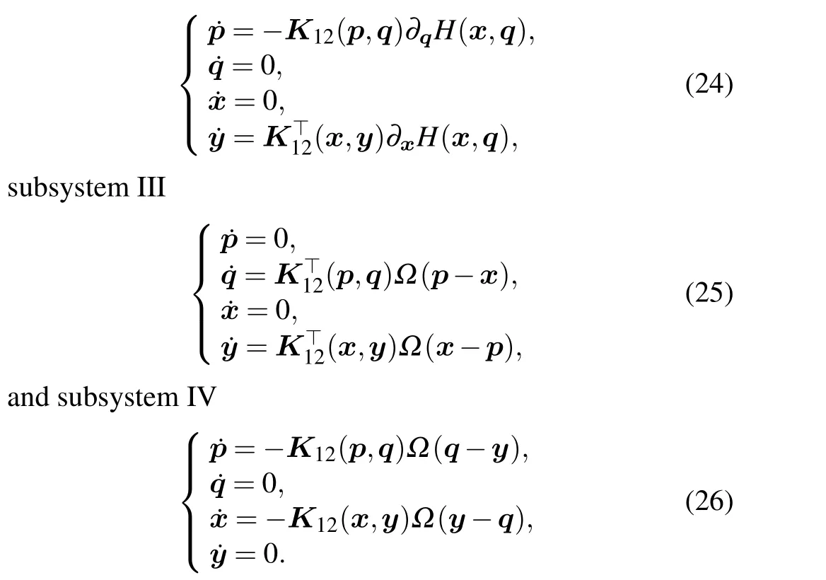
subsystem II The problem is that under which situation,the four subsystems can be solved explicitly and the explicit K-symplectic methods can be constructed.For the above problem, we have the following theorem.
Theorem 1 In the following situation, the above four subsystems(23),(24),(25),and(26)can be solved explicitly.
If the elements
Proof For the proof we refer to the details in Ref.[49].
If all the four subsystems(23)-(26)can be solved explicitly, K-symplectic methods can be constructed by composing the analytical solutions of all the subsystems.To prove this,we simplify the case with just two subsystems.Assume that the HamiltonianHof the non-canonical Hamiltonian system (9)can be split into two parts, i.e.,H=HA+HB, then the system(9)can be separated into two subsystems

which is a second order explicit K-symplectic method.[63]Higher order explicit K-symplectic methods can be constructed by composing the first order K-symplectic method.
Remark 2 For arbitrary two dimensional nonseparable non-canonical Hamiltonian system, the four subsystems can be solved exactly.Thus the K-symplectic methods can be constructed in the extended phase space by composing the exact solution of the four subsystems.
For high dimensional non-separable systems, if the matrixK-1has the special structure as Eq.(18) and satisfies the requirements in the above Theorem 1, then we only need to make two copies of the phase space to construct explicit K-symplectic methods.If the matrix does not have the special structure, we will show another way to construct explicit K-symplectic methods in the next section.
3.Explicit K-symplectic methods for general nonseparable systems
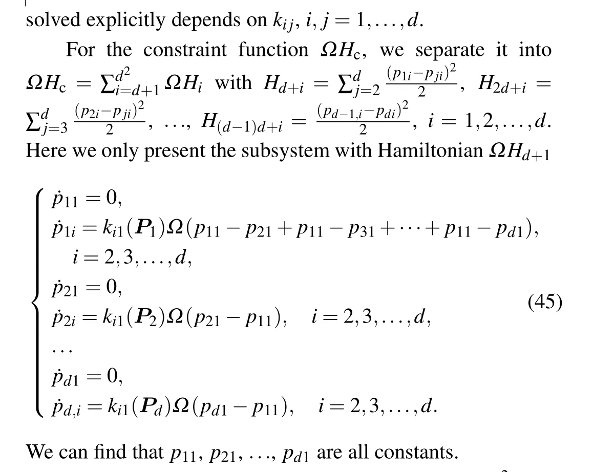
Letd= 2n, we consider theddimensional noncanonical Hamiltonian system (9) with nonseparable HamiltonianH(P)=H(p1,p2,...,pd).The skew-symmetric matrixK-1(Z) has no special structure.Denote byK-1=(ki j)d×d.We extend theddimensional phase space tod2dimensional phase space.Denote byP1=(p11,p12,...,p1d),
P2=(p21,p22,...,p2d),...,Pd=(pd1,pd2,...,pdd).
We first consider the augmented Hamiltonian with mixup variables as follows:
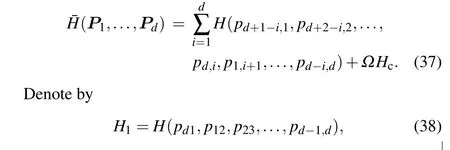

then ¯H=H1+H2+···+Hd+ΩHcfor any 1≤i ≤d,Hitakes one variable fromPj, 1≤j ≤d.The functionHcis a constraint with
Then the new system is
It can be verified that if the conditionsP1(t)=P2(t)=···=Pd(t)hold,the above system(43)is thedcopies of the original system(9),thus we haveP1(t)=P2(t)=···=Pd(t)=P(t)if the same initial condition is imposed onPand eachPi,1≤i ≤d.
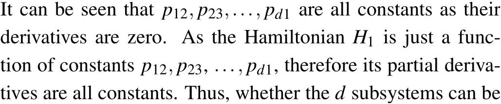
The next step is to explicitly solve each subsystem with the HamiltonianHifor 1≤i ≤d.Here we present the subsystem withH1=H(pd1,p12,p23,...,pd-1,d)
Theorem 3 In the following situation,the aboved2subsystems can be solved explicitly.
If the form of the matrixK-1is under the variable
P=(p1,p2,...,pd)is

Proof For the proof we refer to the details in Ref.[64].
Remark 3 By extending theddimensional phase space to thed2dimensional phase space, whether the subsystems can be solved exactly depends totally on the elements of the skew-symmetric matrixK-1.
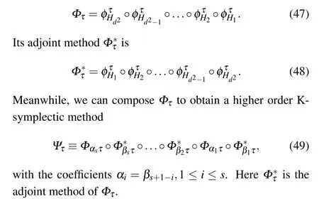
If all thed2subsystems can be solved explicitly,then the first order explicit K-symplectic method can be constructed by composing all the exact solutions.The higher order explicit K-symplectic methods can be constructed by composing the first order K-symplectic method.More specifically,denote the exact solution of each subsystem byφτHi,i=1,2,...,d2and denoteτby the time stepsize,then the first order K-symplectic methodΦτis
In many real problems, the high dimensional problem can be decoupled into several lower dimensional problems,thus one can solve the lower dimensional problems.For example, the equation for the distribution functionfof the Vlasov-Maxwell equations can be rewritten as a 6ndimensional Hamiltonian system by expressingfas a sum of Dirac masses[65]and the 6ndimensional system can be decoupled intoncharged particle systems of 6 dimension.
4.Error analysis
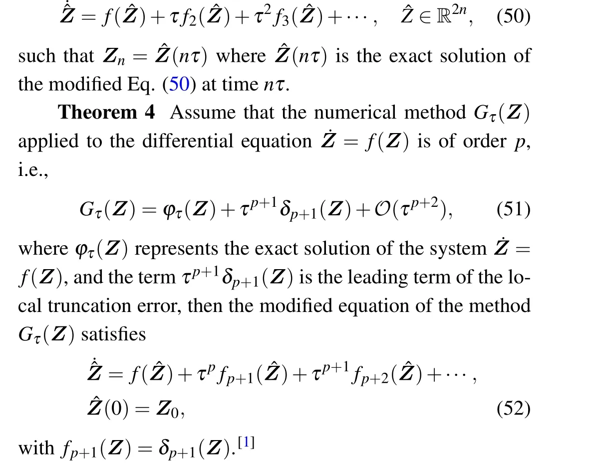
The K-symplectic methods can preserve the K-symplectic structure of the non-canonical Hamiltonian system.Another property of the K-symplectic methods is that they can nearly preserve the Hamiltonian without secular drift over long time.The Hamiltonian of the non-canonical Hamiltonian system is also called the energy of the system.Different from the energy-conserving methods which can exactly preserve the energy,[66-70]the K-symplectic methods only possess near energy conservation property.The near energy conservation property of the K-symplectic methods can be seen from the following theorem.The theory of backward error analysis is the main approach to investigating the long-term behavior of the K-symplectic methods.The main idea of backward error analysis is to view the numerical solution obtained by one numerical method as the exact solution of a new system with a new vector field that is an approximation of the original vector field.More specifically, we assume that a numerical methodGτ(Z) proceeds a series of numerical solutionZi,i=1,2,...,m, whereZiis the value at thei-th time step.Given a differential equation ˙Z=f(Z)and the numerical methodGτ(Z), the idea of backward error analysis is to search for a modified equation
Proof For the proof,please see the proof of Theorem 1.2 of Chapter IX in Ref.[1].
If the differential equation is a non-canonical Hamiltonian system and the method is a K-symplectic method, then we have the following theorem.
Theorem 5 If the numerical methodGτ(Z) of orderpapplied to the non-canonical Hamiltonian system (9) is Ksymplectic,then its modified equation is also a non-canonical Hamiltonian system with the new Hamiltonian ˆH.To be specific, for every initial valueZ0∈R2n, there exists a neighborhoodUand smooth functionsHj:U →R,j=p+1,p+2,...such that the modified equation of the methodGτ(Z)satisfies[1]
the new Hamiltonian ˆH=H+τpHp+1+τp+1Hp+2+···is also called the formal energy ofGτ(Z).
Proof For the proof,please see the proof of Theorem 3.5 of Chapter IX in Ref.[1].
According to Theorem 5,we know that the difference of the HamiltonianHat two adjoint two steps is
As the valuesZnandZn+1calculated by the K-symplectic methodGτ(Z)are the exact solutions of the modified Eq.(53),together with the fact that the Hamiltonian is exactly preserved by the exact solution, then we know that ˆH(Zn+1)= ˆH(Zn).Therefore,we obtain thatH(Zn+1)-H(Zn)=O(hp).


The above error analysis is a rough error estimate,the true error bound may be even smaller.But the error bound provides a constraint on the time stepsize.
5.Numerical experiments
5.1.Numerical methods
To demonstrate the superiority in the structure preservation and efficiency of the K-symplectic methods, we compare them with higher order Runge-Kutta methods, the implicit symplectic methods,the explicit and implicit symplectic methods for the original nonseparable noncanonical Hamiltonians, several other fourth order explicit K-symplectic methods for the extended phase space Hamiltonians, and several fourth order extended phase space K-symplectic-like methods with the midpoint permutation.DenoteΦτby the first order K-symplectic method composed by the exact solution of all subsystems which is defined in Eqs.(34)and(47).
2ndKSYM: the second order K-symplectic method for the extended non-canonical Hamiltonian system,which is the composition ofΦτand its adjoint method isΦ∗τ[63]
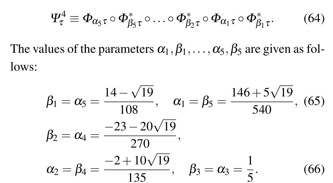
4thKSYM:the fourth order K-symplectic method for the extended non-canonical Hamiltonian system, which is composed by[71]
According to Remark 1,we can prove that both the 2nd-KSYM method and the 4thKSYM method are K-symplectic methods.It should be noticed that both the 2ndKSYM method and the 4thKSYM method are not applied to the original noncanonical Hamiltonian system,thus they are not K-symplectic in the original system.
3rdRK: the third-order explicit Runge-Kutta method(Heun method).[72]It can be applied to both the extended noncanonical Hamiltonian system and the original non-canonical Hamiltonian system.
5thRK: the explicit Runge-Kutta method with effective order 5 (Butcher method).[62,72]It can be applied to both the extended non-canonical Hamiltonian system and the original non-canonical Hamiltonian system.
2ndMIDP: the second-order implicit midpoint rule[27,28]for the original non-canonical Hamiltonian system (9).This method is symmetric and symplectic for the Hamiltonian systems.
2ndSV:the second-order St¨omer-Verlet method[1]for the original non-canonical Hamiltonian system (9).This method is semi-implicit and symmetric.It is also symplectic for the Hamiltonian systems.We denote it bySV2τ.
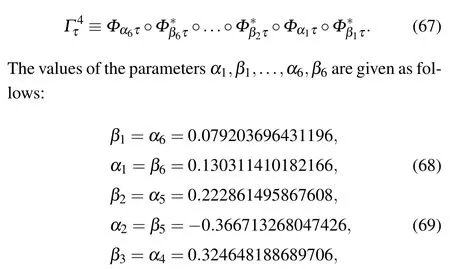
4thBPRK:the optimized fourth-order partitioned Runge-Kutta method for the extended non-canonical Hamiltonian system proposed in Refs.[39,73].The method is composed by
4thYOS: the fourth-order Yoshida’s K-symplectic methods for the extended non-canonical Hamiltonian system.[23]The method is composed by
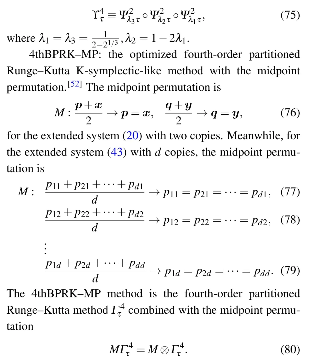
It should be noticed that for the method 4thBPRK-MP, the midpoint permutation is chosen to control the copies of the variables,thusΩis no longer needed,thereforeΩ=0 in the methodΓ4τ.
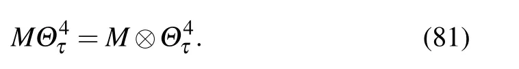
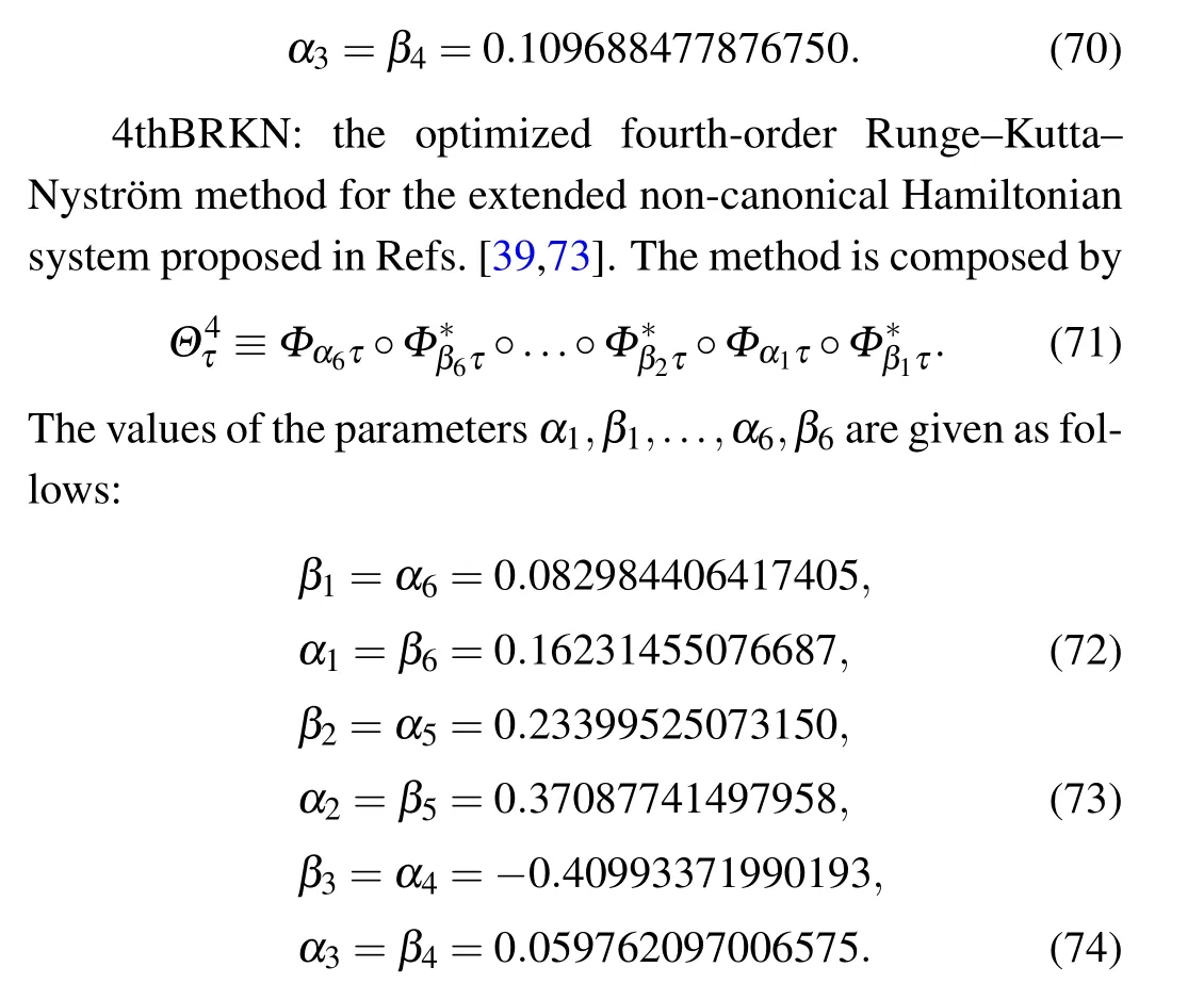
4thBRKN-MP: the optimized fourth-order Runge-Kutta-Nystr¨om K-symplectic-like method with the midpoint permutation.[52]The 4thBRKN-MP method is the fourthorder Runge-Kutta-Nystr¨om methodΘ4τcombined with the midpoint permutation It should be noticed that for the method 4thBRKN-MP, the midpoint permutation is chosen to control the copies of the variables,thusΩ=0 in the methodΘ4τ.
4thYOS-MP: the fourth-order Yoshida’s symplectic-like method with the midpoint permutation.[52]The method is the fourth-order Yoshida’s method Υ4τcombined with the midpoint permutation
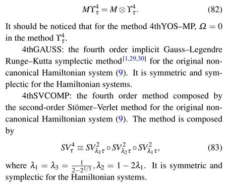
We note here the 2ndMIDP, the 2ndSV, the 4thGAUSS,and the 4thSVCOMP are applied to the original non-canonical Hamiltonian system.As they are implicit or semi-implicit methods, the Newton iteration method is used to solve them.The tolerance error for both second order methods is 1×10-12while the tolerance error for both fourth order methods is 1×10-15.
5.2.The first numerical demonstration for Ablowitz-Ladik model
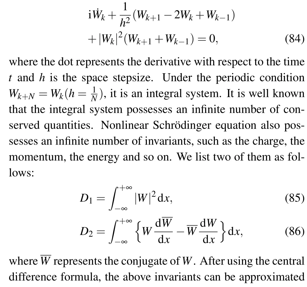
The Ablowitz-Ladik model is one of the space discretization of the nonlinear Schr¨odinger equation[1,74-76]with the form of
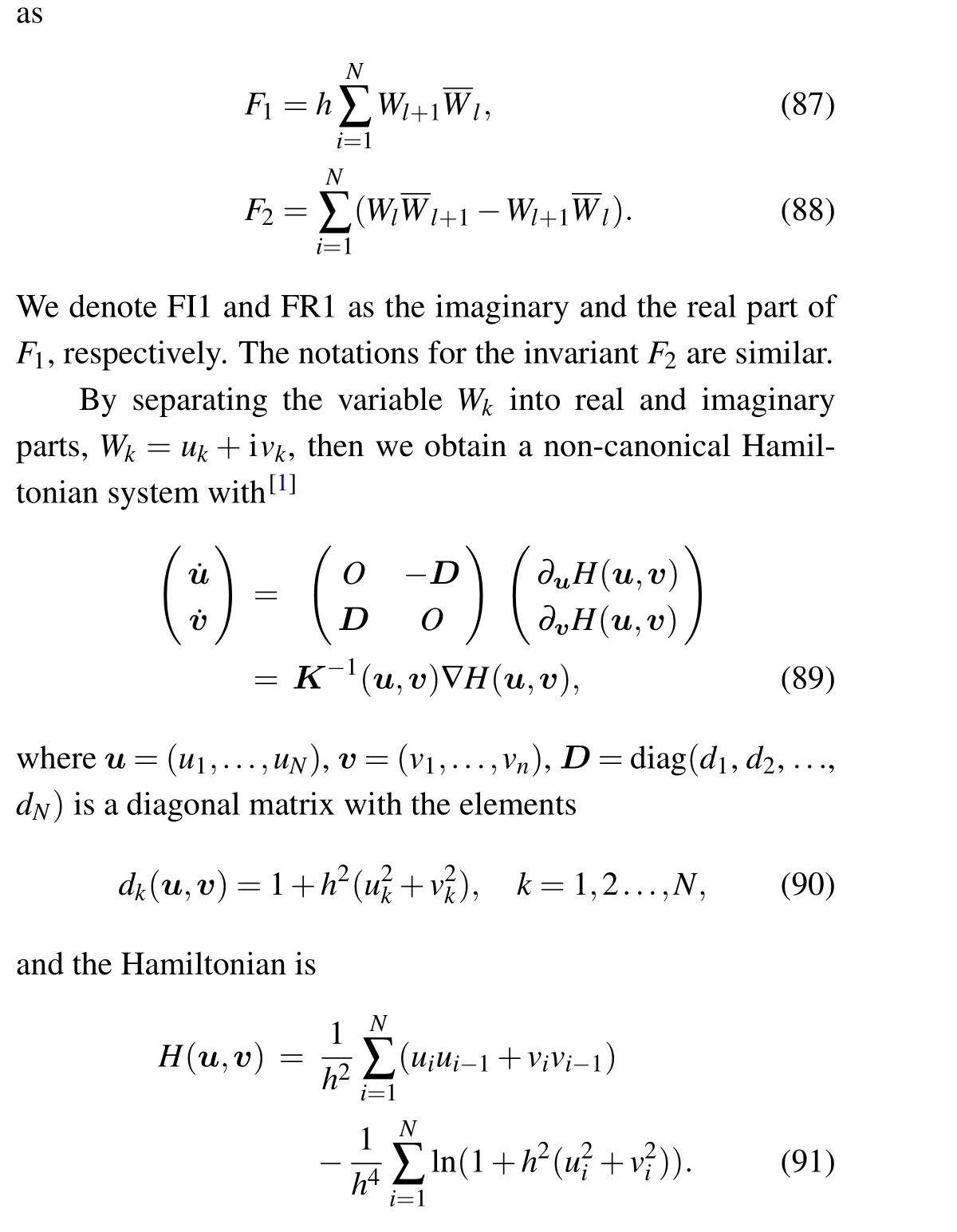
It should be noticed that the pair of variables (ui,vi) is not a pair of canonical variables.We can easily prove that the matrixK-1(u,v)appeared in the system(89)is anti-symmetric,nonsingular, and satisfies the Jacobi-identity, therefore this matrix is aKmatrix.As a result, the system (89) is a noncanonical Hamiltonian system.It can also be seen that the matrixK-1satisfies the requirements in Theorem 1.Thus,we extend the phase space and make the two copies of(u,v).
We takeN=4 and denote the two copies of (u,v) byP=(p1,p2,...,p8) andQ=(q1,q2,...,q8).Thus we consider the augmented Hamiltonian
wherehis the space stepsize andpi0,qi0are the initial values ofpi,qi.As the HamiltonianH1is the function of constantspi0,qi+4,0,i=1,2,3,4,therefore their partial derivatives with respect to its arguments are all constants.The others subsystems can also be solved explicitly,therefore the explicit K-symplectic methods can be constructed by composing the exact solution of all the subsystems.
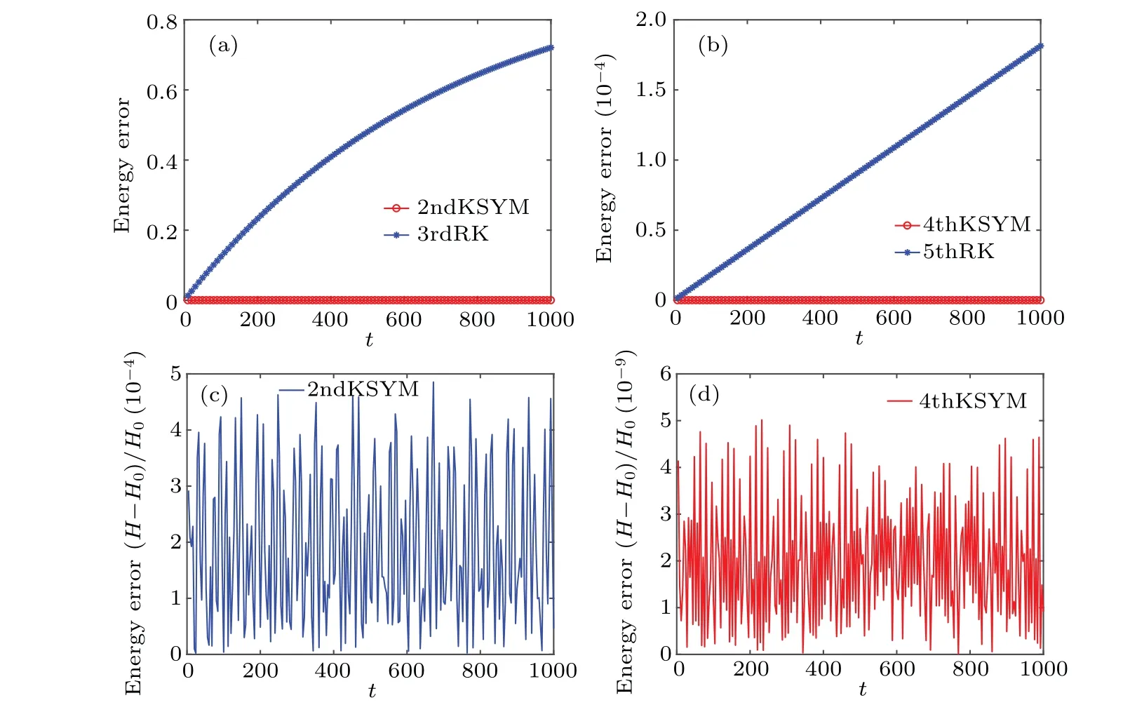
Fig.1.The energy evolutions of the 2ndKSYM method,the 3rdRK method,the 4thKSYM method,and the 5thRK method.Subfigures(a)and(b)display the relative energy error of the augmented Hamiltonian ¯H for the four methods with Ω =20 and the time stepsize τ =0.001.In the first two subfigures the energy error is represented by| ¯H- ¯H0|/| ¯H0|.Subfigures(c)and(d)display the relative energy error of the original Hamiltonian H with Ω =20 and τ =0.001.In the last two subfigures the energy error is represented by|H-H0|/|H0|.
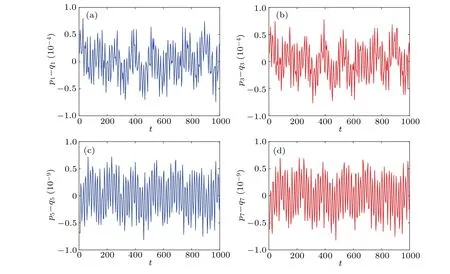
Fig.2.The difference between the two copies for the four variables u1,u3,v1,and v3.Subfigures(a)and(b)display the differences between the two copies for the variables u1 and u3 obtained by the 2ndKSYM method.Subfigures(c)and(d)display the differences between the two copies for the variables v1 and v3 obtained by the 4thKSYM method.Here the time stepsize is τ =0.001 and Ω =20,the final time is T =1000.
The initial condition isu10= 0.2, u20= 0.4, u30=0.3, u40= 0.5,v10= 0.3, v20= 0.2,v30= 0.3, v40= 0.2.The two copies of the variable (u,v) have the same initial condition.The energy evolutions of the augmented Hamiltonian ¯Hobtained by the 2ndKSYM, 4thKSYM, 3rdRK, and 5thRK methods are displayed in Fig.1.The energy errors of the K-symplectic methods oscillate with small amplitudes while the energy errors of the Runge-Kutta methods increase without bound as can be seen from Fig.1.The explicit Ksymplectic methods have shown their significant advantages in energy conservation over long-term simulation compared with the higher order Runge-Kutta methods.The energy errors of the original HamiltonianH(p1,...,p8)in the first copy of variables obtained by the two explicit K-symplectic methods are also shown in Fig.1.As can be seen from Fig.1 that the energy errors can be bounded at very small intervals.This shows that the explicit K-symplectic methods can also preserve the original Hamiltonian over long time.The two copies of the variable(u,v)are also compared.We show the differences between the two copies ofu1, u3, v1, v3in Fig.2.The errors in the two copies ofu1, u3, v1, v3obtained by the two explicit K-symplectic methods are all bounded by small numbers.We display the evolutions of the invariants FI1 and FI2 obtained by the 2ndKSYM method and the 4thKSYM method in Fig.3.As can be seen from Fig.3 that the imaginary part of the invariantsF1andF2are both bounded well over long time.
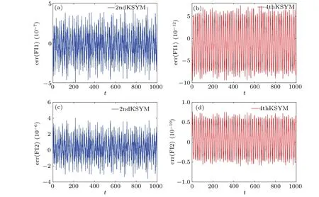
Fig.3.The errors of the invariant FI1 and FI2 obtain by the 2ndKSYM and 4thKSYM methods.The initial value is the two copies of(0.2,0.4,0.3,0.5,0.3,0.2,0.3,0.2), the time stepsize τ =0.001, Ω =20.The error means the difference between the value at each time step and the value at the initial step.

Fig.4.Dependence of the maximal relative energy error on the parameter Ω for the 2ndKSYM method and the 4thBRKN method solving orbits 1,2,and 3.In subfigure(a),the initial values for orbit 1,2,and 3 are two copies of(0.3,0.5,0.1,0.6,0.2,0.3,0.5,0.1),(0.8,0.5,0.6,0.3,0.1,0.4,0.2,0.7),and (0.9,0.5,0.6,0.3,0.2,0.4,0.2,0.7).In subfigure (b), the initial values for orbit 1, 2 and 3 are two copies of (0.1,0.2,0.3,0.4,0.5,0.6,0.7,0.8),(0.2,0.2,0.3.0.4,0.6,0.7,0.8,0.9),and(0.6,0.7,0.8,0.9,0.1,0.2,0.3,0.4).Obviously,in subfigure(a)Ω =32 is an appropriate choice while in subfigure(b)Ω =4 is an appropriate choice.
As the control parameterΩis dependent on the algorithms and the initial conditions.We plot the dependence of the maximal relative energy error on the parameterΩfor both the 2ndKSYM method and the 4thBRKN method when solving three orbits in Fig.4.The three orbits correspond to three different initial conditions.It is shown in Fig.4(a) thatΩ=32 is an appropriate choice for the 2ndKSYM method.Thus, one of the initial condition in Fig.4(a) and the chosenΩare used to compare the computational efficiency of the 2ndKSYM method,the 2ndMIDP method,and the 2ndSV method.The results are shown in Fig.5(b).It is also shown in Fig.4(b)thatΩ=4 is an appropriate choice for the 4thBRKN method.One of the initial condition in Fig.4(b)and the chosenΩare used to compare the computational efficiency of all the fourth-order methods and the results are shown in Figs.5(c)and 5(d).
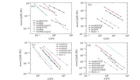
Fig.5.The log-log plot for the computational efficiency for each method over the interval[0,T].In subfigure(a),the time stepsize τ for the 2ndKSYM and 3rdRK method is τ=0.001/2i,i=0,1,2,3,the τ for the 4thKSYM and 5thRK method is τ=0.008/2i,i=0,1,2,3,the initial value is(0.2,0.4,0.3,0.5,0.3,0.2,0.3,0.2),Ω =20 and T =100.In subfigure(b),the time stepsize τ for the three methods is τ =0.001/2i,i=0,1,...,4,the initial value is(0.3,0.5,0.1,0.6,0.2,0.3,0.5,0.1),Ω =32 and T =100.In subfigures(c)and(d),the time stepsize τ for these methods is τ =0.008/2i,i=0,1,2,3,the initial value is(0.1,0.2,0.3,0.4,0.5,0.6,0.7,0.8),Ω =4 and T =100.
Figure 5 shows the computational efficiency of all the methods listed in the Subsection 5.1.Figure 5(a)displays the computational efficiency of the 2ndKSYM,the 4thKSYM,the 3rdRK, and the 5thRK method.It is shown that under the time stepsizeτ=0.001, the energy error of the 2ndKSYM method is about six orders of magnitude smaller than that of the 3rdRK method.Under all the stepsizes, the energy errors of the 2ndKSYM method are much smaller than those of the 3rdRK method.The CPU time of the 2ndKSYM method is a bit bigger than that of the 3rdRK method applied to the extended non-canonical Hamiltonian system.The energy errors of the 3rdRK method applied to the original system and the extended system are nearly the same, while the CPU time of the 3rdRK method applied to the original system is less.It can also be seen that the energy errors of the 4thKSYM method are also much smaller than those of the 5thRK method under all the stepsizes.The reason why the energy error of the 2ndKSYM method at the top point is less than that of the 4thKSYM method at the top point is that the time stepsize for the 2ndKSYM method is much less.And the reason why we choose larger stepsizes for the 4thKSYM method is to clearly show the order of the method.Figure 5(a)shows that the K-symplectic methods exhibit much better energy behavior than the higher order Runge-Kutta methods.Figure 5(b)shows the computational efficiency for the three second order methods.One method is said to be more efficient than the other method if it takes less CPU time to obtain the same order magnitude of error.As is shown in Fig.5(b)that to obtain the same energy error, like 10-6, the CPU time of the 2nd-KSYM method is much less than those of the 2ndMIDP and the 2ndSV methods.This shows that the 2ndKSYM method is more efficient than the 2ndMIDP method and the 2ndSV method.The computational efficiency of all the fourth-order methods are displayed in Figs.5(c)and 5(d).As can be seen from Fig.5(c)that although the energy error of the 4thKSYM method is larger than that of the 4thBPRK method at the same stepsize,but to obtain the same order magnitude of energy error,the CPU time of the 4thKSYM method is less than that of the 4thBPRK method.This shows that the 4thKSYM method is more efficient than the 4thBPRK method.The energy error of the 4thKSYM method is nearly the same as that of the 4thBRKN method, but its CPU time is less than that of the 4thBRKN method.This also exhibits that the 4thKSYM method is more efficient than the 4thBPRK method.When we compare the 4thKSYM method with the 4thBPRK-MP method and the 4thBRKN-MP method, the CPU time of the 4thKSYM method is larger than those of the two methods,but the energy error of the 4thKSYM method is slightly small.The reason why the 4thKSYM method takes more CPU time is that the number of subsystems is two times of the 4thBPRKMP and the 4thBRKN-MP methods.Displayed in Fig.5(d)is the comparison between the 4thKSYM method and the others fourth order methods.As can be seen from Fig.5(d) that the 4thKSYM method can not only obtain less energy error,but also take less CPU time than the 4thGAUSS,the 4thYOS,the 4thYOS-MP,and 4thSVCOMP methods.This shows that the 4thKSYM method exhibits much better efficiency than the others four methods.
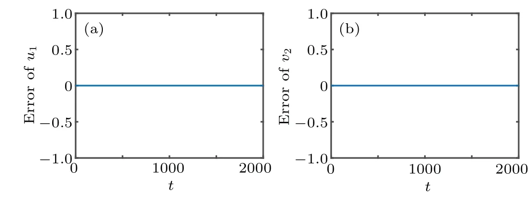
Fig.6.The error of variables u1 and v2 between solution in the original phase space and that in the extended phase space.The initial value is (0.2,0.4,0.3,0.5,0.3,0.2,0.3,0.2) and Ω =20.Subfigure (a) displays the error between the original u1 and the first copy of u1,subfigure(b)displays the error between the original v2 and the second copy of v2.
We also plot the errors between the solution in the original phase space and that in the extended phase space in Fig.6.The initial value of the extended system is the two copies of the original ones.The both solutions are calculated by using the ode45 function in Matlab.The relative tolerance and the absolute tolerance are set to be 10-12and 10-12,respectively.As can be seen from Fig.6 that there is no difference between the solution in the original phase space and that in the extended phase space for the Ablowitz-Ladik model.
5.3.The second numerical demonstration for gyrocenter system
Gyrocenter system[8-10]plays a fundamental role in plasma physics research.Many neoclassical phenomena in tokamak experiments,such as the bootstrap current,are underlied by gyrocenter dynamics.As is mentioned above,the gyrocenter motion is obtained by averaging out the fast gyromotion from the charged particle dynamics.It is a non-canonical Hamiltonian system
wherepi0,qi0,ri0,wi0represent the initial values ofpi,qi,ri,wifori=1,2,3,4.As the HamiltonianH1is the function of the constantsp1,q2,r3,w4,therefore the partial derivative ofH1with respect to each argument is also a constant.The others subsystems can also be solved explicitly, thus the explicit K-symplectic methods can be constructed.
The initial condition isx0=0.003,y0=0.002,z0=0.004 andu0=0.005.The four copies of the original variablesx,y,z,uhave the same initial condition.The orbits inp1-p2plane obtained by the 2ndKSYM method and the 3rdRK method are

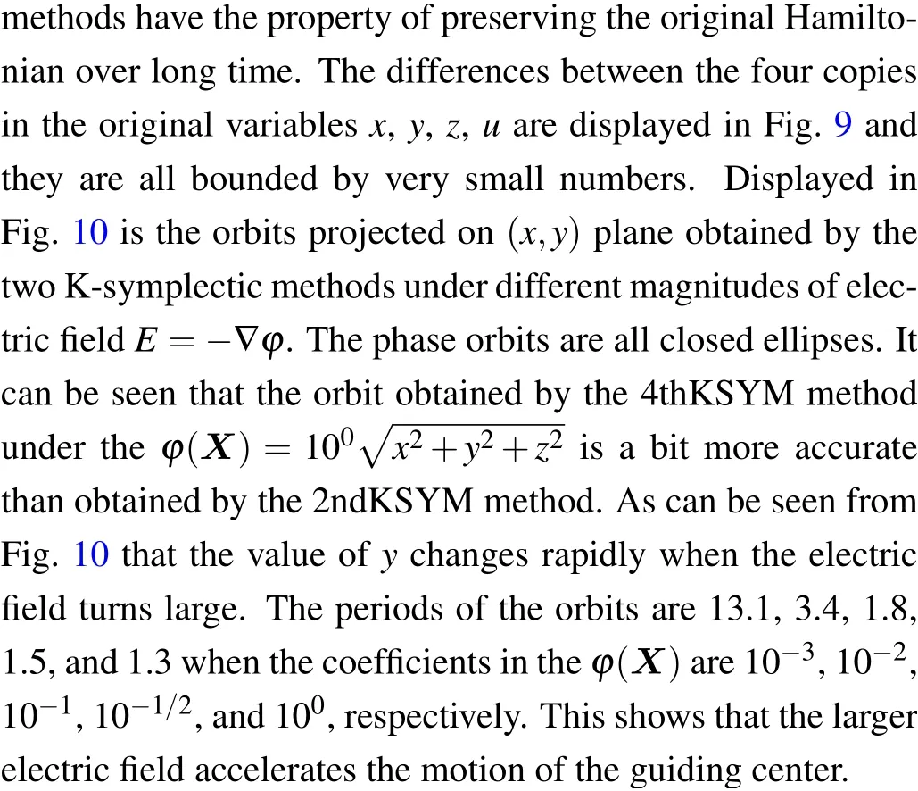
Fig.7.The phase orbit and the energy error obtained by the 2ndKSYM method, the 3rdRK method, the 4thKSYM method, and the 5thRK method.Subfigures (a) and (b) display the orbit projected to p1-p2 plane obtained by the 2ndKSYM method and the 3rdRK method with stepsize τ=0.01,Ω=20 over the time interval[0,10000].Subfigures(c)and(d)display the relative energy error of the augmented Hamiltonian¯H for the four methods with Ω =20.In subfigure(c),the stepsize τ =0.01/4 while in subfigure(d)τ =0.01.The energy error is represented by| ¯H- ¯H0|/| ¯H0|.
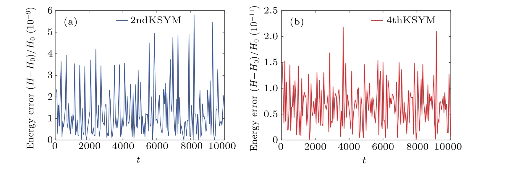
Fig.8.The relative energy error of the original Hamiltonian H(p1,p2,p3,p4)obtained by the 2ndKSYM method and the 4thKSYM method.The relative energy error is represented by(H-H0)/H0.The stepsize is chosen as τ =0.01 and the parameter is Ω =20.
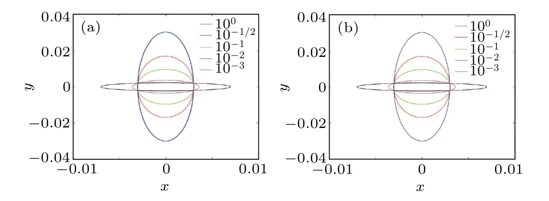
Fig.10.The phase orbit obtained by the 2ndKSYM and the 4thKSYM methods under different electric field.The initial condition is(0.003,0.002,0.004,0.005),Ω =20 and T =100.The coefficient in the φ(X)varies from 10-3 to 100.Subfigure(a)is the result obtained by the 2ndKSYM method while subfigure(b)is the result obtained by the 4thKSYM method.
Figure 11 shows the dependence of the maximal relative energy error on the parameterΩfor the 2ndKSYM method and the 4thBPRK method when solving three orbits.The three orbits correspond to three different initial conditions.It is shown in Fig.11(a) that the energy error is nearly the same no matter how big theΩis, thus we chooseΩ=18.One of the initial condition in Fig.11(a) and the chosenΩare used to compare the computational efficiency of the 2nd-KSYM method,the 2ndMIDP method,and the 2ndSV method and the results are shown in Fig.12(b).As can be seen from Fig.11(b)thatΩ=6 is an appropriate choice for the 4thBPRK method.One of the initial condition in Fig.11(b) and the chosenΩare used to compare the computational efficiency of all the fourth-order methods and the results are shown in Figs.12(c)and 12(d).
Figure 12 shows the computational efficiency of all the numerical methods.Figure 12(a) displays the computational efficiency of the 2ndKSYM, the 4thKSYM, the 3rdRK, and the 5thRK method.It is shown that to obtain the same order magnitude of energy error, the CPU time of the 2nd-KSYM method is less than that of the 3rdRK method applied to the extended phase space Hamiltonian.Thus the 2ndKSYM method is more efficient than the 3rdRK method applied to the extended phase space Hamiltonian.It can also be seen from Fig.12(a) that the 4thKSYM method is more efficient than the 5thRK method applied to the extended phase space Hamiltonian.The K-symplectic methods are less efficient than the higher-order Runge-Kutta methods applied to the original non-canonical Hamiltonian system.Figure 12(b) shows the computational efficiency for the three second order methods.As shown in Fig.12(b)that the energy error of the 2nd-MIDP method is less than that of the 2ndKSYM method at each time stepsize.But to obtain the same order magnitude of error, like 10-10, the CPU time of the 2ndKSYM method is less than that of 2ndMIDP method.This exhibits that the 2nd-KSYM method is more efficient than the 2ndMIDP method.As shown in Fig.12(b)that the 2ndKSYM method is more efficient than the 2ndSV method.The computational efficiency of all the fourth order methods are displayed in Figs.12(c)and 12(d).It can be seen from Fig.12(c) that the 4thKSYM method is more efficient than the 4thBPRK method and the 4thBRKN method.It is also shown in Fig.12(c) that both the energy error and the CPU time of the 4thBPRK-MP and the 4thBRKN-MP methods are less than those of 4thKSYM methods.The reason why the 4thKSYM method takes more CPU time is that more subsystems are required to be calculated.Thus,the 4thBPRK-MP method and the 4thBRKN-MP method are more efficient than the 4thKSYM method.Displayed in Fig.12(d)is the comparison between the 4thKSYM method and the others fourth order methods.As can be seen from Fig.12(d) that the 4thKSYM method is more efficient than the 4thGAUSS method and the 4thYOS method.Furthermore, the energy error of the 4thKSYM method is much less than that of the 4thYOS method under the same stepsize.On the other hand, although at the same stepsize, the energy error of the 4thKSYM method is about two orders of magnitude smaller than that of the 4thYOS-MP method, but the CPU time of the 4thKSYM method is nearly four times of the 4thYOS-MP method.This is because the 4thYOS-MP method calculates less subsystems and only need triple composition ofΨ2τ.Figure 12(d) also shows that the 4thKSYM method exhibits much better efficiency than the 4thSVCOMP method.
We also plot the errors between the solution in the original phase space and that in the extended phase space in Fig.13.The initial value of extended system is the four copies of the original ones.The both solutions are calculated by using the ode45 function in Matlab.The relative tolerance and the absolute tolerance are set to be 10-12and 10-12, respectively.Figure 13 shows that the errors in two variables between the solution in the original phase space and that in the extended phase space are bounded by the machine precision.
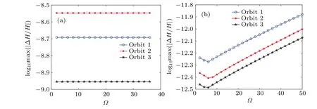
Fig.11.Dependence of the maximal relative error on the parameter Ω for the 2ndKSYM method and the 4thBPRK method solving orbits 1, 2, and 3.In subfigure (a), the initial values for orbit 1, 2, and 3 are four copies of (0.03,0.05,0.05,0.06), (0.05,0.06,0.05,0.08),and (0.07,0.03,0.02,0.04).In subfigure (b), the initial values for orbit 1, 2, and 3 are four copies of (0.0005,0.0006,0.0005,0.0007),(0.0005,0.0007,0.0005,0.0007),and(0.0006,0.0007,0.0005,0.0008).Obviously,in subfigure(b)Ω =6 is an appropriate choice.
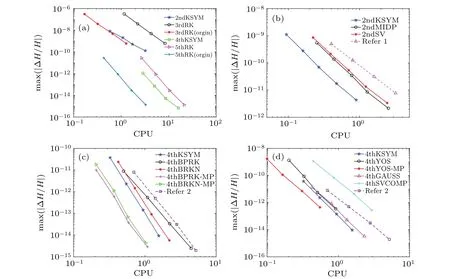
Fig.12.The log-log plot for the computational efficiency for each method over the interval[0,T].In subfigure(a), the time stepsize τ for the four methods is τ =0.002/2i,i=0,1,2,3,the initial value is(0.003,0.002,0.004,0.005),Ω =20,and T =2000.In subfigure(b),the time stepsize τ for the three methods is τ =0.001/2i,i=0,1,...,4,the initial value is(0.07,0.03,0.02,0.04),Ω =18,and T =100.In subfigures(c)and(d),the time stepsize τ for these methods is τ =0.002/2i,i=0,1,2,3,the initial value is(0.0005,0.0006,0.0005,0.0007),Ω =6,and T =100.
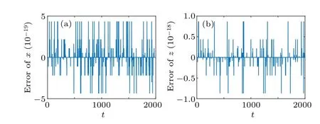
Fig.13.The error of variables x and z between solution in the original phase space and that in the extended phase space.The initial value is(0.003,0.002,0.004,0.005)and Ω =20.Subfigure(a)displays the error between the original x and the first copy of x,subfigure(b)displays the error between the original z and the second copy of z.
6.Conclusion
We propose explicit K-symplectic methods for noncanonical Hamiltonian systems with nonseparable Hamiltonian.The idea is to extend the original phase space to several copies of the phase space and to impose a mechanical restraint on the copies of the phase space.Explicit K-symplectic methods have been constructed for two non-separable noncanonical Hamiltonian systems and are compared with higher order explicit Runge-Kutta methods.The numerical results show that the K-symplectic methods have superiority in phase orbit tracking and energy conservation over long-term simulation compared with the higher order Runge-Kutta methods.The differences between the several copies of the variables are also bounded by the K-symplectic methods.The numerical results also show that the 2ndKSYM method is more efficient than the 3rdRK applied to the extended systems,the 2ndMIDP method and the 2ndSV method applied to the original systems.Meanwhile, the 4thKSYM method is more efficient than the 5thRK applied to the extended systems,the 4thBPRK and the 4thBRKN methods for the extended systems and the 4thYOS,the 4thGAUSS,and the 4thSVCOMP methods for the original systems.The energy error of the 4thKSYM method is much less than those of the 4thYOS and the 4thYOS-MP methods under the same time stepsize.The numerical results also show that the 4thKSYM method is less inferior to the 4thBPRKMP and 4thBRKN-MP in efficiency because less subsystems are required be calculated in the latter two methods, but their energy errors are nearly in the same magnitude.Thus, the 2ndKSYM method and the 4thKSYM method are suitable for long-time simulations of nonseparable noncanonical Hamiltonian systems.
Acknowledgement
Project supported by the National Natural Science Foundation of China(Grant Nos.11901564 and 12171466).
猜你喜欢
杂志排行

Chinese Physics B的其它文章
- Matrix integrable fifth-order mKdV equations and their soliton solutions
- Comparison of differential evolution,particle swarm optimization,quantum-behaved particle swarm optimization,and quantum evolutionary algorithm for preparation of quantum states
- Molecular dynamics study of interactions between edge dislocation and irradiation-induced defects in Fe-10Ni-20Cr alloy
- Engineering topological state transfer in four-period Su-Schrieffer-Heeger chain
- Spontaneous emission of a moving atom in a waveguide of rectangular cross section
- Novel traveling quantum anonymous voting scheme via GHZ states