Yan GAO, Jiali FENG, Xin XIA, Jian SUN, Yulong MA, Dongmei CHEN, and Qilin WAN*

1Guangdong-Hong Kong-Macao Greater Bay Area Weather Research Center for Monitoring Warning and Forecasting, Shenzhen 518038, China

2CMA Earth System Modeling and Prediction Centre, China Meteorological Administration, Beijing 100081, China

ABSTRACT In the traditional incremental analysis update (IAU) process, all analysis increments are treated as constant forcing in a model’s prognostic equations over a certain time window.This approach effectively reduces high-frequency oscillations introduced by data assimilation.However, as different scales of increments have unique evolutionary speeds and life histories in a numerical model, the traditional IAU scheme cannot fully meet the requirements of short-term forecasting for the damping of high-frequency noise and may even cause systematic drifts.Therefore, a multi-scale IAU scheme is proposed in this paper.Analysis increments were divided into different scale parts using a spatial filtering technique.For each scale increment, the optimal relaxation time in the IAU scheme was determined by the skill of the forecasting results.Finally, different scales of analysis increments were added to the model integration during their optimal relaxation time.The multi-scale IAU scheme can effectively reduce the noise and further improve the balance between large-scale and small-scale increments in the model initialization stage.To evaluate its performance, several numerical experiments were conducted to simulate the path and intensity of Typhoon Mangkhut (2018) and showed that: (1) the multi-scale IAU scheme had an obvious effect on noise control at the initial stage of data assimilation; (2) the optimal relaxation time for large-scale and small-scale increments was estimated as 6 h and 3 h, respectively; (3) the forecast performance of the multiscale IAU scheme in the prediction of Typhoon Mangkhut (2018) was better than that of the traditional IAU scheme.The results demonstrate the superiority of the multi-scale IAU scheme.

Key words: multi-scale incremental analysis updates, optimal relaxation time, 2-D discrete cosine transform,GRAPES_Meso, Typhoon Mangkhut (2018)

1.Introduction

In terms of spatial coverage, numerical models can be classified into two major categories: global models and regional models.Both have unique advantages in describing analysis information at different scales.Because global analysis is not affected by biases at lateral boundaries, the largescale aspect of global analysis is superior to the aspect of regional analysis (Peng et al., 2010; Zhuang et al., 2020).However, after assimilating observation data with high spatial density, the regional analysis may yield a more accurate small-scale analysis (Zhuang et al., 2018).To improve the forecasting performance of a regional model, one possible approach is to use a blending technique, which includes an incremental spatial filter to blend large-scale analysis from the global model with small-scale fields from the high-resolu-tion regional model (Denis et al., 2002; Yang, 2005; Hsiao et al., 2015).

Although the advantages of the blending technique have been collectively presented by some previous studies(Keresturi et al., 2019; Feng et al., 2021), this method still has some limitations in short-term forecasts, such as shortterm precipitation climatology, likely owing to the imbalance between large-scale analysis from the global model and small-scale analysis from the regional model (Polavarapu et al., 2004; Schwartz et al., 2021).To further improve the performance of the blending technique, it is necessary to employ some strategies to combat this imbalance.One effective method to accomplish this task is to apply an incremental analysis update (IAU) technique.Bloom et al.(1996) first proposed the IAU technique, which gradually incorporated the analysis increment.Since this technique emerged, it has been widely used in the atmospheric and oceanic fields and is considered to be successful in keeping the mass and momentum fields in dynamic balance by removing spurious gravity waves (Ourmières et al., 2006; Zhang et al., 2015;Lei and Whitaker, 2016).

In a traditional IAU scheme, the background system is considered to be linearly evolving over a given time window.Therefore, the traditional IAU scheme has a fixed time window, which is called the relaxation time, τ (Xu et al.,2019; Li et al., 2021).All analysis increments are gradually incorporated into the model integration during the relaxation time (Chen et al., 2020).However, in real weather processes,different scales of incremental analyses are produced by corresponding scales of weather systems, which have unique evolutionary speeds, life histories, and response times.Compared with large-scale information, small-scale information evolves more rapidly and has a shorter life history in the regional model.However, both large- and small-scale increments have the same time window in the traditional IAU method, which cannot entirely represent the propagation characteristics of information having different scales.

To remedy the shortcomings of the traditional IAU technique and improve the forecast performance of the numerical model, this paper proposes a multi-scale IAU scheme for the first time.Through the blending method, the analysis increments were divided into two categories, large- and small-scale increments.Several IAU experiments were designed to determine the optimal relaxation time (ORT)for each scale increment.Using the multi-scale IAU scheme,different scales of analysis increment were added into model integration during their own ORT, and the corresponding forecast performance was evaluated in the prediction of Typhoon Mangkhut (2018).

The remainder of this paper is structured as follows.Section 2 describes the methodology used in detail.The model configuration and the numerical experiments conducted in this study are introduced in section 3.The differences in the simulation results between different kinds of IAU schemes in Typhoon Mangkhut (2018) are analyzed in section 4.Finally, a discussion and conclusion are given in section 5.

2.Methodology

The typhoon initialization scheme proposed in this paper is based on the multi-scale IAU technique.There are three main steps to achieve the initialization scheme.First,through the 3DVAR system, the background field in the regional model is transformed into a 3DVAR analysis field.Then, the blended analysis field, which consists of largescale analysis information obtained from the global analysis field and small-scale analysis information obtained from the 3DVAR analysis field, is obtained through the blending method, with a spectral transform called the two-dimensional discrete cosine transform (2D-DCT) (Denis et al., 2002).Finally, by using the multi-scale IAU technique, the largescale and small-scale analysis increments are incorporated into the integration of the regional model over their own time windows.The blending method and the IAU scheme are introduced in detail in the following sections.

2.1.Blending Method

As mentioned in section 1, the regional model has more accurate small-scale analysis information than the global model.However, the solution obtained from the regional and global models is inconsistent.This inconsistency may produce unexpected noise and cause instabilities owing to wave reflection along the lateral boundaries (Davies, 1983).Therefore, systematic large-scale errors can be made in the limited domain, leading to a distortion of large-scale information in the regional model after a significant period of integration (Peng et al., 2010).A blending method is applied in the regional model to solve this problem.

In the regional model, the background field and the 3DVAR analysis field are designated asGxbandGxa, respectively.Then, the incremental analysis betweenGxbandGxais expressed asGdxa.Moreover, the global analysis field obtained from NCEP GFS analysis is defined asGglobal.Through the 2D-DCT blending method, the blended analysis fieldGblndcan be calculated as:

whereFfilter,Lis a low-pass spatial filter with a spectral transform called 2D-DCT.The filter cutoff length adopted in the blending method is chosen as 600 km, which is guided by the GRAPES-RAFS, a rapid analysis and forecast system operated at the Center of Numerical Weather Prediction,CMA (Zhuang et al., 2020).

As shown in Eq.2, the blended analysis incrementGdblndis obtained asGblnd-Gxb, which includes the largescale increment, Δl=Ffilter,Land the smallscale increment, Δs=Gdxa-Ffilter,L(Gdxa).It follows:

2.2.Multi-scale IAU Method

To reduce the high-frequency oscillations induced by the analysis increment, different types of IAU methods are widely applied in atmospheric models.The basic principle of IAU is to gradually incorporate an increment calculated from the analysis during the model integration.In the IAU scheme, analysis increments are treated as constant additional forcing terms in the model’s prognostic equations over a certain time window (relaxation time, τ):

whereFis the prognostic variable, ··· represents the increment introduced by the model integration, andFaandFbare the analysis and background fields, respectively.

The IAU scheme called three-dimensional IAU(3DIAU) uses a single increment that is assumed to be constant over an assimilation window during model integration.In contrast to 3DIAU, the propagation of the increment information over an assimilation window is considered in fourdimensional IAU (4DIAU).Time-varying analysis increments are gradually incorporated into the model integration through 4DIAU (Lorenc et al., 2015; Lei and Whitaker,2016).

Regardless of which type of IAU scheme is adopted, all scales of analysis increments are incorporated in the model integration over the same time window.However, different scales of incremental information have different evolutionary speeds and life histories in the regional model, which cannot be represented by the traditional IAU method.

In this section, based on the principle of the IAU technique, a first proposal of the multi-scale IAU technique is outlined.In the multi-scale IAU scheme, different scales of analysis increments are added to the model integration over different time windows:

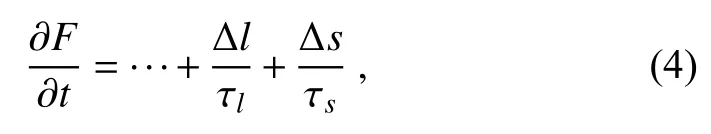
where Δland τlare the large-scale analysis increment and its relaxation time, respectively, while Δsand τsrepresent the small-scale analysis increment and its relaxation time,respectively.

Figure 1 shows the schematic illustration of two different categories of IAU schemes.The blue area above the coordinate axis represents the traditional IAU technique, and τ is the relaxation time.The red area below the coordinate axis displays the multi-scale IAU scheme, in which the largescale increment and small-scale increment are incorporated into the model integration over the time windows τland τs,respectively.

3.Model Configurations and Experimental Design

3.1.Model Configuration

The numerical weather prediction model used in this study is the mesoscale version of the Global/Regional Assimilation and PrEdiction System (GRAPES_Meso), which is a new generation of numerical weather forecasting systems for mesoscale weather prediction developed by the China Meteorological Administration (CMA) (Chen and Shen,2006).The model adopts a height-based terrain-following coordinate, a semi-implicit and semi-Lagrangian (SI-SL)time difference scheme, a fully compressible non-hydrostatic balance dynamic framework, and a physical parameterization package (Wu et al., 2005; Chen et al., 2008).The physical parameterization schemes selected in this study include the rapid radiative transfer model (RRTM) for the long-wave scheme (Rosenkranz, 2003), the Dudhia shortwave radiation scheme (Dudhia, 1996), the WRF single-moment six-class(WSM6) microphysics scheme (Hong and Lim, 2006), the Noah land surface scheme, the Monin-Obukhov surface layer scheme (Johansson et al., 2001), and the mediumrange forecast (MRF) planetary boundary layer scheme(Hong and Pan, 1996).

The model uses a single domain, which covers the area 15°-30°N, 104°-122.9°E, with a horizontal grid spacing of 3 km (6 31×501 grid points) and 51 vertical layers reaching up to 33 km.The time step of the model is 30 s.The initial and lateral boundary conditions are obtained from NCEP GFS analyses at 0.25° resolution.

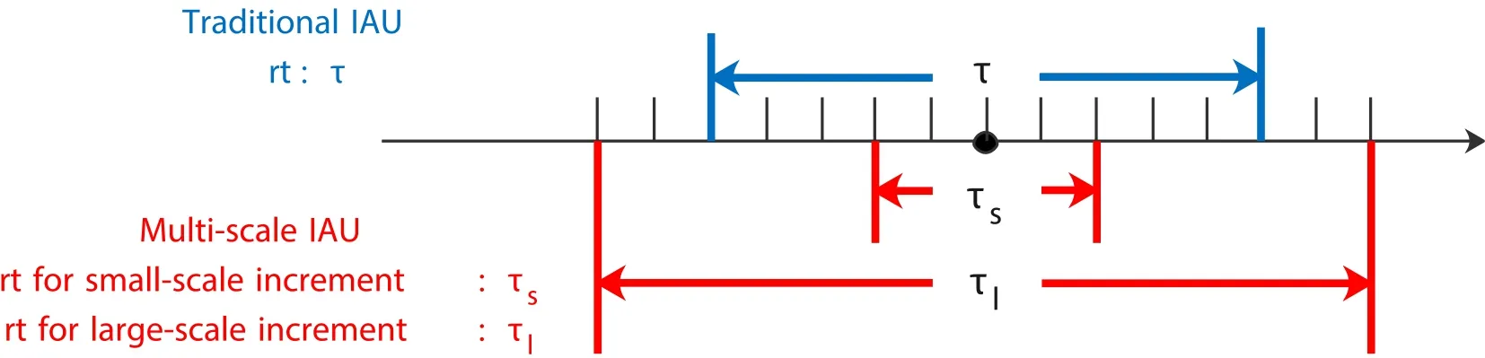
Fig.1.Illustration of two IAU schemes.The blue area is the traditional IAU technique, of which the relaxation time is τ.The red area is the multi-scale IAU approach, and the relaxation times of the large-scale and small-scale increments are τl and τs, respectively.The abbreviation for relaxation time is rt in the figure.

3.2.Experimental design

Some numerical experiments were designed to evaluate the performance of the multi-scale IAU scheme.The blending experiment, illustrated in red in Fig.2, was first designed to ensure that the regional model derived a physically valid state after initialization (Ulmer and Balss, 2016).The background field was integrated from the initial condition of the regional model and downscaled from the global analysis at(t0-6)h, with a 6 h warm-up time.Then, the background fieldGxbat the analysis timet0was generated.The GRAPES_Meso 3DVAR (Xue et al., 2008) and the blending method were successively applied att0.The Gaussian correlation model was used in the GRAPES_Meso 3DVAR system.The horizontal correlation length of specific humidity was shorter at 200 km, while that of the other variances was 500 km.The 3DVAR analysis fieldGxaatt0was obtained by using the 3DVAR system.After that, the 2-D DCT blending method mentioned in section 2.1 was immediately performed to obtain the blended analysis fieldGblndatt0.Specifically, the large-scale analysis increment from NCEP GFSGglobaland the small-scale analysis increment from the 3DVAR analysis fieldGxawere blended to create the blended analysis increment.After the background fieldGxbwas replaced by the blended analysis fieldGblnd, the model performed a 36-h continuous forecast.

In addition to the blending experiment, the IAU experiment was also designed and presented in blue in Fig.2.The background field was integrated from the global analysis field at (t0-6)h, and the increment obtained from the blending experiment was treated as constant forcing in a model’s prognostic equation through the IAU scheme over the time window (t0-τ/2,t0+τ/2).Here, the center of the time windows was att0, and the relaxation time was τ.Aftert0, the model performed a 36-h continuous forecast.

For the IAU scheme, the relaxation time, τ, is a crucial parameter that determines the filtering properties of the analysis increments.IAU experiments with different configurations were designed to test initialization sensitivity to relaxation time and find the optimal relaxation time (ORT) for each scale increment.In the seven large-scale IAU experiments, the large-scale increment was added into the integration at every time step over different relaxation times in Typhoon Mangkhut (2018).The CMA tropical cyclone (TC)database was chosen to verify the TC track and intensity forecasts (Ying et al., 2014; Lu et al., 2021).Based on the verified results, the ORT of the large-scale increment could be determined.Similarly, seven small-scale IAU experiments were also designed to obtain the ORT of the small-scale increment.For the multi-scale IAU experiment, the relaxation times of the large- and small-scale increments were derived from the ORTs of the large-scale and small-scale IAU experiments, respectively.Finally, three all-scale IAU (traditional IAU) experiments and a control experiment (without IAU)were also conducted to evaluate the performance of the multi-scale IAU scheme.Table 1 shows the configuration of all numerical experiments in detail.

4.Analysis of results

4.1.Description of case study

In this paper, Typhoon Mangkhut (2018) was chosen as a case study.Mangkhut (2018) was the strongest typhoon to make landfall in China in 2018.It formed as a tropical depression on 7 September 2018 before moving westward and intensifying into a typhoon.On 15 September 2018, it first battered Cagayan, Philippines, and on 16 September 2018, it made a second landfall in Jiangmen, Guangdong Province, China,as an approximately 900-km-wide super typhoon with a central minimum pressure of 955 hPa and maximum sustained winds of 42 m s-1at 0900 UTC.

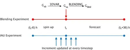
Fig.2.Illustration of two categories of numerical experiments, which included the blending experiment (red lines) and the IAU experiment (blue lines).In the blending experiment, the background field G xb was integrated from the global analysis field at (t0-6) h, and the 3DVAR and blending methods were successively applied at the analysis time t0 to obtain the blended analysis field G blnd.In the IAU experiment, the background field was also integrated at (t0-6) h, and the increment, which was calculated in the blending experiment, was added to the integration at every time step during the time window.Both the blending experiment and the IAU experiment performed a 36-h continuous forecast after t0.

For the Mangkhut (2018) case, 20 comparison experiments with different initialization schemes were conducted(Table 1).According to the model domain shown in Fig.3,the background field, in this case, was first integrated from the global analysis field at 0000 UTC on 15 September 2018, which is presented as the red dot in Fig.3.After 6-h of spin-up time, the analysis time (t0) was 0600 UTC on 15 September 2018 (blue dot in Fig.3).For the blending experiment, the blended analysis increments were obtained by using the 3DVAR and blending methods.In this work, the atmospheric motion vectors (AMVs) derived from the infrared channel (IR1) and water vapor channel (IR3) of the satellite FY-2G were assimilated by the GRAPES_Meso 3DVAR.The temporal and spatial resolutions of the observation data were 6 h and 5 km × 5 km, respectively.The distribution of AMVs shows that 90% of the observation data were high-level winds (above 399 hPa), while the middlelevel (400-699 hPa) and low-level winds (below 700 hPa)accounted for 8% and 2%, respectively.The arrows corresponding to the wind vectors in Fig.3 represent the distribution of high-level winds.In this case, the small-scale increment was only added to the wind field, while the large-scale increment, obtained from the global model, was applied to wind, pressure, water vapor mixing ratio, and potential temperature.Figure 4a shows the wind in the background field at the 200-hPa layer att0, and Figs.4b-c display the large-and small-scale wind increments at 200 hPa, respectively.Aftert0, the model performed a 36-h continuous forecast with outpout every 6-h and ended its simulation at 1800 UTC on 16 September 2018, a timestamp represented by the black dot in Fig.3.

Table 1.Configuration of 20 numerical experiments.

Fig.3.The domain of the GRAPES_Meso adopted in this work and the CMA best track and intensity of Typhoon Mangkhut (2018) from 0000 UTC on 15 September to 1800 UTC on 16 September 2018.The numerical experiments began at the red dot and ended at the black dot.The red arrow of wind vectors represents the distribution of high-level winds (above 399 hPa)derived from FY-2G at the analysis time t0, which is denoted by the blue dot.

Fig.4.(a) Wind in the background field, (b) large-scale, and (c)small-scale wind increments at the 200-hPa layer.All wind fields were obtained at 0600 UTC on 15 September 2018 (t0).

4.2.Optimal Relaxation Time for IAU Scheme

Seven large-scale IAU (LS_IAU) and seven small-scale IAU (SS_IAU) experiments were conducted to find the optimal relaxation time in the IAU scheme.The simulation results were analyzed in detail.

4.2.1.Large-scale IAU Experiment

Among all large-scale experiments, there was one experiment that did not adopt the IAU scheme (LS_No_IAU),which means that the large-scale increment was completely incorporated into the model integration att0.The other six LS_IAU experiments used the IAU scheme, with relaxation times of 0.5 h, 1.0 h, 1.5 h, 3.0 h, 6.0 h, and 9.0 h, respectively.For comparison, the simulation result of the control(CTL) experiment is also presented in this section.

The average tendency of the surface pressure can be used as an indicator of the noise level in the external gravity wave component.Figure 5 displays the average tendency of the surface pressure in the CTL experiment and seven LS_IAU experiments.Note that the presented surface pressure tendency was area-averaged over the whole domain and output every 10 min.The red dashed curve represents the surface pressure of LS_No_IAU, of which the peak value reached over 1 hPa (10 min)-1att0.Throughoutt0to(t0+4)h, the surface pressure of LS_No_IAU was evidently larger than that of the other curves.Excessive noise, presented by the red dashed curve, indicates the obvious presence of gravity waves, and the spin-up time here was estimated to be 4 h.The other six solid lines represent LS_IAUs with different relaxation times.The results show that IAU schemes were important in removing high-frequency noise, and larger relaxation times were associated with lower noise levels.Because there was no analysis increment introduced,the surface pressure tendency of CTL, shown as the black dashed line in Fig.5, was minimal.

The track errors between the simulated track and the CMA best track versus time are presented in Fig.6a.Overall, the track error between the observation and forecast results increased with time.The mean track error in each experiment is shown in Fig.6b.The mean values ranged from 55.6 km to 69.5 km, and the minimum appeared in the experiment with a relaxation time of 6 h (LS_IAU_6h).Compared with CTL, the mean track error of LS_IAU_6h was reduced by about 21%.

The minimum sea level pressure (MSLP) at the typhoon center was the simple measure of intensity for Typhoon Mangkhut (2018).Figure 7a displays the intensity errors between the forecast and observation results and shows that the simulated MSLP was larger than observed att0.After a 12-h forecast, the simulated MSLP became smaller than the observation data, and the intensity errors increased with time.Figure 7b shows the mean values of the intensity errors obtained from CTL and seven large-scale IAU experiments.The mean intensity errors ranged from 11 to 12.1 hPa, and the minimum value was also obtained from LS_IAU_6h.Compared with CTL, the intensity error of LS_IAU_6h was reduced by about 9.1%.

After comprehensively considering the track and intensity errors presented in this section, the optimal relaxationtime for LS_IAU in Typhoon Mangkhut (2018) was 6 h.

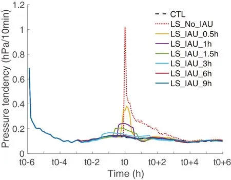
Fig.5.Surface pressure tendency versus time.The black and red dashed lines represent CTL and LS_No_IAU, respectively.The other six solid curves are the simulation results of large-scale IAU experiments with different relaxation times.The surface pressure tendency was area-averaged over the whole domain, with output every 10 min.

4.2.2.Small-scale IAU Experiment

Similar to the LS_IAU experiments, seven small-scale IAU (SS_IAU) experiments were also conducted.One of them was without the IAU scheme (SS_No_IAU).While the other six applied the IAU technique, and their relaxation times were 0.5 h, 1.0 h, 1.5 h, 3.0 h, 6.0 h, and 9.0 h, respectively.

Figure 8 displays the average tendency of the surface pressure in eight experiments.The red dashed curve, representing SS_No_IAU, illustrates the obvious presence of spurious gravity waves introduced by the small-scale analysis increment.The surface pressure caused by the small-scale increment was smaller than that caused by the large-scale increment.Moreover, some high-frequency oscillations occurred in the SS_IAU experiments, and the spin-up period of SS_No_IAU was about 5 h.The solid lines in Fig.8 show that the IAU technique effectively removed these noises.

The typhoon track error versus time is presented in Fig.9a.The track error in each experiment showed a slight decrease in the first 6 h and then gradually increased with time.Figure 9b shows the mean values of the track errors in CTL and the seven SS_IAU experiments.These ranged from 66.6 km to 70.8 km, and the minimum error was obtained from SS_IAU_3h.Compared to CTL, the mean track error of SS_IAU_3h was reduced by about 4.2%.

Figure 10a shows the intensity errors versus time in the CTL and SS_IAU experiments.Aftert0, the simulated MSLPs were smaller than observations.Figure 10b presents the mean values of the intensity errors simulated by CTLand seven SS_IAU experiments.The mean intensity errors had a small range, between 12.1 and 12.5 hPa; for the SS_IAU experiments, SS_IAU_3h had a minimal intensity error, essentially the same as the CTL.The mean values of the intensity errors obtained from the other six SS_IAU experiments were slightly larger than CTL.Such results imply that introducing a small-scale analysis increment produces little improvement in typhoon intensity forecasts.In this case,the optimal relaxation time for SS_IAU was determined to be 3 h.

Fig.8.Surface pressure tendency versus time.The black and red dashed lines represent CTL and SS_No_IAU, respectively.The other six solid curves are the simulation results of SS_IAUs with different relaxation times.

Fig.9.(a) Track errors of Typhoon Mangkhut (2018) versus time and(b) the mean values of track error in CTL and the seven small-scale increment experiments.

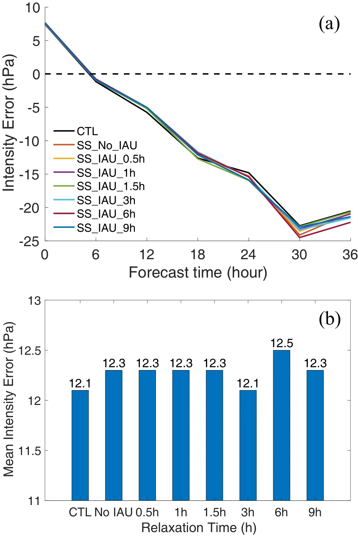
Fig.10.(a) Intensity errors of Typhoon Mangkhut (2018) versus time and (b)the mean intensity errors in CTL and seven small-scale IAU experiments.

4.3.Best Forecast Results

The simulation results of the large- and small-scale IAU experiments indicated that the optimal relaxation times for LS_IAU and SS_IAU in Case Mangkhut (2018) were 6 h and 3 h, respectively.Therefore, the best initialization scheme of MS_IAU was the 6-h relaxation time for the large-scale increment and the 3-h relaxation time for the small-scale increment.For comparison, the all-scale IAU experiments with three different relaxation times (1 h, 3 h,and 6 h) were also considered.Eight numerical experiments were compared to test the performance of different IAU schemes on both typhoon path and intensity.These eight experiments included the CTL experiment, the BLND experiment, the best LS_IAU experiment (LS_IAU_6h), the best SS_IAU experiment (SS_IAU_3h), three AS_IAU experiments (AS_IAU_1h, AS_IAU_3h, and AS_IAU_6h), and the MS_IAU experiment (MS_IAU_6h&3h).

Figure 11a shows the track errors versus time for the eight numerical experiments.Throughout the 36-h integration period, almost all categories of numerical experiments had an increasing trend of track errors with time, and the values of track errors ranged from 12.7 to 169.8 km.The mean values of track errors are presented in Fig.11b, which shows a mean track error of CTL of 69.5 km, representing the maximum among the eight experiments.In addition to CTL, theresults of the three experiments with IAU initialization were larger than those of the BLND experiment; among them was SS_IAU_3h.We suppose that this is mainly caused by two factors 1) compared to the large-scale environmental flow field, the small-scale increment field itself had little effect on the typhoon track performance, and 2) the vertical distribution of the small-scale increment adopted in this case was uneven.Notably, 90% of the small-scale increment consisted of high-level winds (above 399 hPa), while the small-scale, incremental information below 399 hPa was scarce and scattered.Therefore, such information was not sufficient enough to represent the characteristics of the smallscale increment field at medium and low levels.

Fig.11.(a) Track errors of Typhoon Mangkhut (2018) versus time and (b) the mean track errors in different categories of numerical experiments.

Although both the large-scale and small-scale increments were incorporated into the model integration in three AS_IAU experiments, the track errors of AS_IAUs with relaxation times of 1 h and 3 h were larger than that of BLND.In contrast, the track performance of AS_IAU_6h was better than that of BLND.The comparative results imply that the track performance was extremely sensitive to the relaxation time of the IAU technique.If the relaxation time was inappropriate, the IAU scheme could even negatively affect the forecast.The minimum track error was 52.5 km, obtained by the MS_IAU_6h&3h.Compared with the CTL, the track errors of MS_IAU_6h&3h decreased by 24.4%.It was also reduced by about 4% in comparison to AS_IAU_6h.

To further analyze the relationship between the observation and simulation tracks of Typhoon Mangkhut (2018) in detail, four groups of Mangkhut (2018) tracks in the 42-h integration process are illustrated in Fig.12.The red line is obtained from the CMA best track data, while the blue,green, and pink lines represent the typhoon tracks simulated in the CTL, BLND, and MS_IAU_6h&3h experiments,respectively.Compared with the best track, all simulated typhoon tracks made a delayed landfall in China.We surmise that the physical characteristics of GRAPES_Meso may be the main reason for this phenomenon.

Figures 13a-b illustrate the intensity errors versus time and the mean values of the intensity errors in eight numerical experiments.Their intensity errors had a range of -24.9 to 7.7 hPa.Att0, the simulated MSLPs were larger than the observation.Aftert0, the simulated MSLP graduallybecame smaller than the observation, and the difference between the simulation and observation intensities increased with time.

Fig.12.Track of Typhoon Mangkhut (2018) from 0000 UTC on 15 September to 1800 UTC on 16 September 2018.The red line is based on the CMA best track of Typhoon Mangkhut (2018), while the blue, green, and pink lines represent the track results obtained from the CTL, BLDN, and MS_IAU_6h&3h experiments, respectively.

It can be seen from Fig.13b that the mean intensity errors obtained from SS_IAU_3h, AS_IAU_1h, and AS_IAU_3h were larger than those of CTL, which means there may be a negative effect on intensity performance if the analysis increment is incorporated into the model through the IAU technique with an inappropriate time window.It is obvious from Fig.13b that the large-scale analysis increment could improve the performance of the typhoon intensity.Compared with CTL, the mean intensity error of LS_IAU_6h was decreased by 9.2%.Although the smallscale wind increment itself did not play an obvious role in improving the simulated typhoon intensity, the mean values of intensity errors of both AS_IAU_6h and MS_ISU_6h&3h were 0.2 hPa lower than those of LS_IAU_6h.

In addition, to further evaluate the performance of the MS_IAU scheme, we compared the forecast results against an independent analysis of the operational ECMWF at 0.25°.For four experiments (CTL, BLND, AS_IAU_6h, and MS_IAU_6h&3h), the RMSEs of horizontal winds, U and V, were calculated between the model analyses and the ECMWF analyses, and the vertical profiles of the mean RMSEs are shown in Figs.14a-b.It can be seen from Fig.14 that the mean RMSE of CTL (pink line) and BLND(yellow line) was clearly larger than that of AS_IAU_6h(red line) and MS_IAU_6h&3h (blue line) for both U and V.The mean RMSE of MS_IAU_6h&3h was slightly smaller than that of AS_IAU_6h for analysis of U, while the RMSE of analysis V was nearly the same for MS_IAU_6h&3h and AS_IAU_6h.

5.Discussion and Conclusion

To prevent spurious high-frequency gravity waves caused by analysis increments, the IAU technique is applied in the numerical model.In the traditional IAU scheme, all scales of analysis increments are treated as constant additional forcing terms in the model’s prognostic equations during the same relaxation time (τ).However, because different scales of analysis information have different evolutionary speeds and life histories in the model, the traditional IAU scheme has some drawbacks.For this reason, this paper first proposes the multi-scale IAU scheme applying different scales of analysis increments, each having optimal relaxation times in the multi-scale IAU method.

To find the optimal scheme for the multi-scale IAU technique and further compare the effects of the traditional and multi-scale IAU schemes, 20 numerical experiments with different configurations were conducted.In the experimental design, Typhoon Mangkhut (2018) was selected as the simulation focus, and the 3DVAR and 2D-DCT blending methods were used successively to obtain large- and small-scale analysis increments, respectively.After analyzing and discussing the results of 20 experiments in detail, we arrived at the following conclusions:

1) For the IAU technique, relaxation time is a crucial parameter.To find the optimal relaxation time for the largescale increment, seven large-scale IAU (LS_IAU) experiments were conducted.One of them was without the IAU method (LS_No_IAU), and the other six were with IAUschemes, but their relaxation times were different.The surface pressure tendency of LS_No_IAU was about six times larger than that in the CTL experiment, which means that the large-scale increment introduced obvious gravity waves.The surface pressure tendency in the other six LS_IAUs was obviously smaller than that in LS_No_IAU, which indicates that the IAU technique played an important role in combating gravity waves.When a 6-h relaxation time was selected, both the track and intensity forecasts of Typhoon Mangkhut (2018) were the best.Compared to CTL, the track and intensity errors of LS_IAU_6h were reduced by about 21% and 9.8%, respectively.Therefore, we regarded 6 h as the optimal relaxation time in the large-scale IAU experiments.

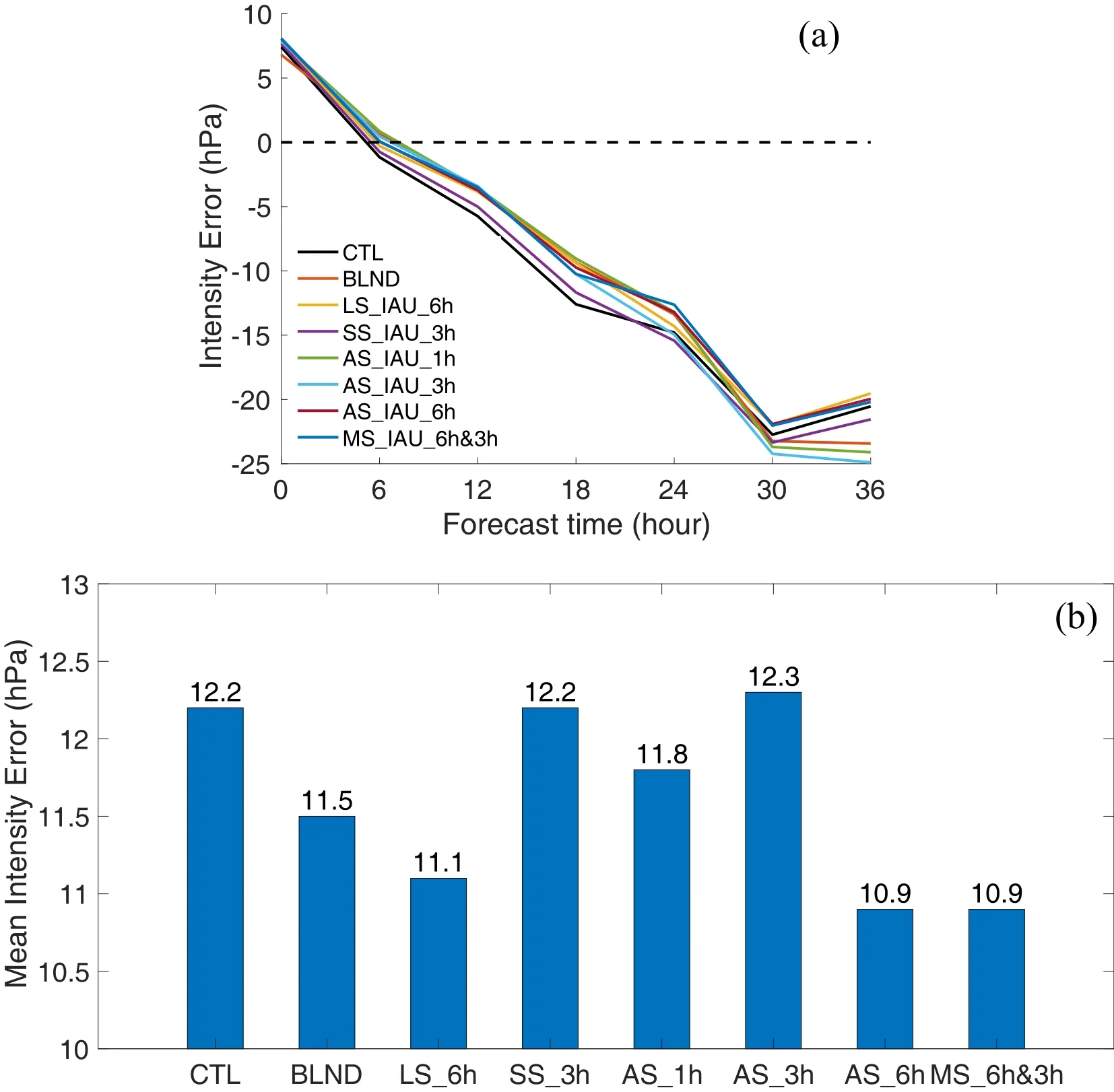
Fig.13.(a) Intensity errors of Typhoon Mangkhut (2018) versus time and (b) the mean intensity errors in different categories of numerical experiments.

2) Similar to the LS_IAU experiments, seven smallscale IAU (SS_IAU) experiments were also presented.One of them was without IAU (SS_No_IAU), and the other six had different relaxation times in IAU schemes.The surface pressure tendency of SS_No_IAU indicated that the smallscale increment also introduced obvious gravity waves.Compared to CTL, the track errors and intensity errors of smallscale increment experiments did not show obvious improvement.The simulation results of some numerical experiments were even worse than those of CTL.We infer that this is due to the vertical distribution of the observation data.The small-scale increment adopted in this case was assimilated from the atmospheric motion vectors (AMVs), only 10% of which was distributed below 399 hPa, so AMVs could not fully reveal the characteristics of the small-scale information below 400 hPa, which is the main reason some SS_IAU experiments exerted a negative effect on the forecast performance.However, some SS_IAUs also showed positive effects on the track error of Typhoon Mangkhut (2018).Among all SS_IAU experiments, the forecast results of SS_IAU_3h were the best.Compared to CTL, the track error of SS_IAU_3h was reduced by 4.2%, and the intensity error was the same.Finally, the optimal relaxation time for the SS_IAU experiment was determined to be 3 h for TyphoonMangkhut (2018).

Fig.14.Vertical profile of the mean analysis RMSEs of (a) U and (b) V for the CTL experiment (pink line),the BLND experiment (yellow line), AS_IAU_6h (red line), and MS_IAU_6h&3h (blue line).

3) For the multi-scale IAU scheme, the relaxation times of the large- and small-scale increments were selected as 6 h and 3 h, respectively.Moreover, another three traditional IAU experiments with different relaxation times were conducted for comparison purposes.The simulation results show that the track error of Typhoon Mangkhut (2018) in MS_IAU_6h&3h was the smallest.Compared with CTL,the mean track error in MS_IAU_6h&3h decreased by 24.5%.Compared to AS_IAU_6h (the best simulation result in the traditional IAU schemes), the result obtained from the MS_IAU experiment was reduced by about 4%.The mean values of the intensity error in AS_IAU_6h and MS_IAU_6h&3h were equal, which was approximately 9.7%less than CTL.Moreover, the mean RMSE of the zonal wind, U, was smallest for MS_IAU_6h&3h, while that for the meridional wind, V, was nearly the same for MS_IAU_6h&3h and AS_IAU_6h.

Overall, among all initialization schemes, the forecasting performance of MS_IAU_6h&3h was the best, which shows the superiority of the multi-scale IAU scheme.In future work, we plan to perform statistical work focusing on the optimal cutoff length and relaxation time for the multiscale IAU technique.

Acknowledgements.This research was jointly sponsored by the Shenzhen Science and Technology Innovation Commission(Grant No.KCXFZ20201221173610028) and the key program of the National Natural Science Foundation of China (Grant No.42130605).The model data in this study are available upon request from the authors via gaoyan@gbamwf.com.