Ya-Dong Huang(黄亚冬) Jia-Wei Fu(付佳维) and Long-Miao Chen(陈龙淼)

1Jiangsu University,Zhenjiang 212013,China

2Nanjing University of Science and Technology,Nanjing 210094,China

Keywords: electromagnetic actuator,backward-facing step flow,flow instability,flow control

1. Introduction

The liquid metal is widely utilized in the thermal management and energy storage due to its high thermal conductivity,[1,2]such as heat exchange in nuclear engineering,[3]cooling of high-power-density microdevices,[4]and harvesting the low grade heat to generate electricity.[5]Also, the liquid metal is attractive in the mechanical to electrical energy conversion via magnetohydrodynamics (MHD) generator[6]due to its excellent electoral conductivity. In the heat transfer flow system, both the heat transfer efficiency and the flow instability are commonly taken into consideration. Usually, a backward-facing step (BFS) is designed in the heat exchanger to enhance the heat transfer via flow separation and reattachment.[7,8]The BFS flow often contains two separation bubbles and the flow structures are mainly dependent on the Reynolds numbers based on the maximum inlet velocity and the hight of the step.[9]Perturbations could gain energy amplification when flowing through the separation bubbles owing to the Kelvin–Helmholtz (KH) instability,[10]Taylor–G¨ortler instability,[11]centrifugal instability[12]and other instability mechanisms,[13,14]and the amplification may make a great influence on the heat transfer efficiency.[15,16]Thereby, researchers adopt active[17,18]and passive[19,20]controls of the BFS flow to achieve the desired heat transfer efficiency. However, the perturbation amplification may aggravate the flow system instability, which is unfavourable for the liquid metal transport. It is an available strategy that the control method could regulate the perturbation energy in the liquid metal BFS flow.

As a classical law of physics, the interactions between the electrical current and the magnetic field in the liquid metal could generate the Lorentz force to control the flow[21,22]and transport the liquid metal.[23]In former studies, the Lorentz force had made great contributions to drag reduction, transition suppression and so forth in the flow control. The Lorentz force is generated by the electromagnetic field which could be excited via the electromagnetic actuator consisting of alternatively arranged electrodes and magnetic poles, and having two types: tile and stripe.[24]The tile-type electromagnetic actuator (TEA) and stripe-type electromagnetic actuator (SEA) could engender the wall-normal and wall-parallel Lorentz force respectively. It was found the streamwise (or wall-parallel) Lorentz force applied in the separation bubble could reduce the bubble size thus modifying the growth rates of the perturbation energy.[25]Moreover, the perturbation energy in the BFS flow also could be adjusted by the linear control model with a feed-forward controller.[26,27]Although research has proposed several control methods to adjust the instability in the BFS flow, the flexibility for different control strategies needs further discussion. Hence,the control effects of different control strategies on the instability in the liquid metal BFS flow would be investigated in this paper.

2. Methodology

The incompressible liquid metal flow controlled via the Lorentz force is modelled by the Navier–Stokes equation:

while the linear evolution of perturbations can be predicted by solving the following linear perturbation equation:

containing the external forcing termℱϑϑand the Lorentz forceℱqq.ℱqandℱϑare the spatial structures of the body force, andqandϑare time-dependent variables representing the noise source and control input respectively.

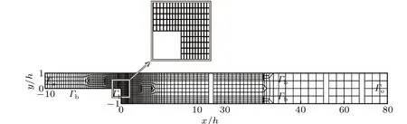
According to the achievements in Refs. [25,26], three control strategies: the base flow control (BFC), linear model control (LMC) and their combination (combined model control,CMC)are considered to adjust the flow instability in this paper. The control model is shown in Fig.1. The step height ishwhich is also the characteristic length. The height of the expansion channel is 2h. To be convenient for description and calculation, the origin of the Cartesian coordinate locates on the step corner. As the Reynolds number in current research is 500,the uncontrolled steady flow contains the primary separation bubble (PSB) on the lower wall and the secondary separation bubble(SSB)on the upper wall.x1is the reattachment point of PSB, andx2,x3are the separation and reattachment points of SSB.

It could be observed that three electromagnetic actuators(A1,A2,and A3)and two sensors(S1and S2)exist in the flow system. According to our previous investigation,[25]SEAs A1and A2could be installed inside the separation bubbles in BFC.TEA A3is applied to LMC which also has the sensors S1and S2. The sensor S1is placed near the noise source to measure the incoming disturbance becauseϑis very difficult to come by in physical experiments. The sensor S2is employed to measure the outputs.

Fig.1. Control model.

In LMC and CMC, the linear control model could be established based on the numerical data of Eq. (2) via the Galerkin projection. As the BFS flow usually acts as a noise amplifier, the Galerkin-based method has many limitation in accurately capturing the transfer behavior from the input to the output.Some researchers adopted the auto-regressive movingaverage exogenous (ARMAX) model[28]to perform the system identification. For simplicity, researchers usually formulate the state-space system in a discrete-time format.The mapping of the inputss,qfrom S1,A3,and the outputmfrom S2could be described by the following model:

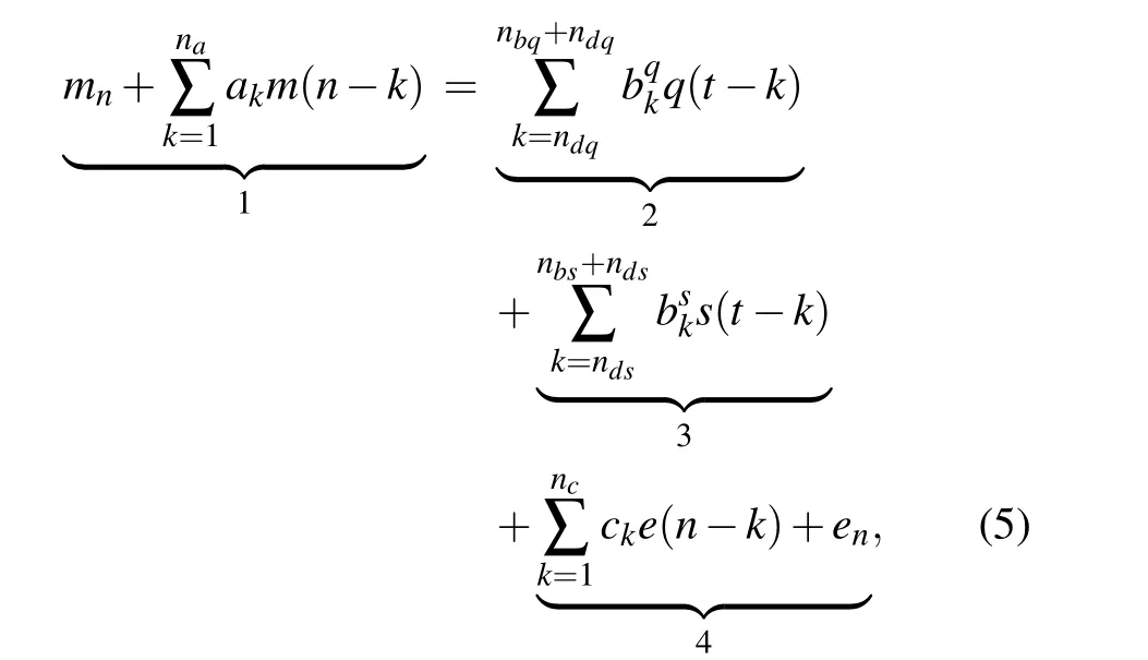
wheremis the output and term 1 is the auto-aggressive part.qandsare the inputs and terms 2,3 represent the exogenous part.eis the noise and term 4 means the moving average part.The coefficientsak,bk, andckcould be found via regression.nais the previous outputs on which the current output depend on.ndqandndsrepresent the numbers of the passed inputs due to the delaying effects of the input on the output.nbqandnbsmean the numbers of the previous inputs on which the current output depends.ncis the number of time-colored noise.Readers could know more about the detailed meaning of the parameters in Eq.(5)in Ref.[26].

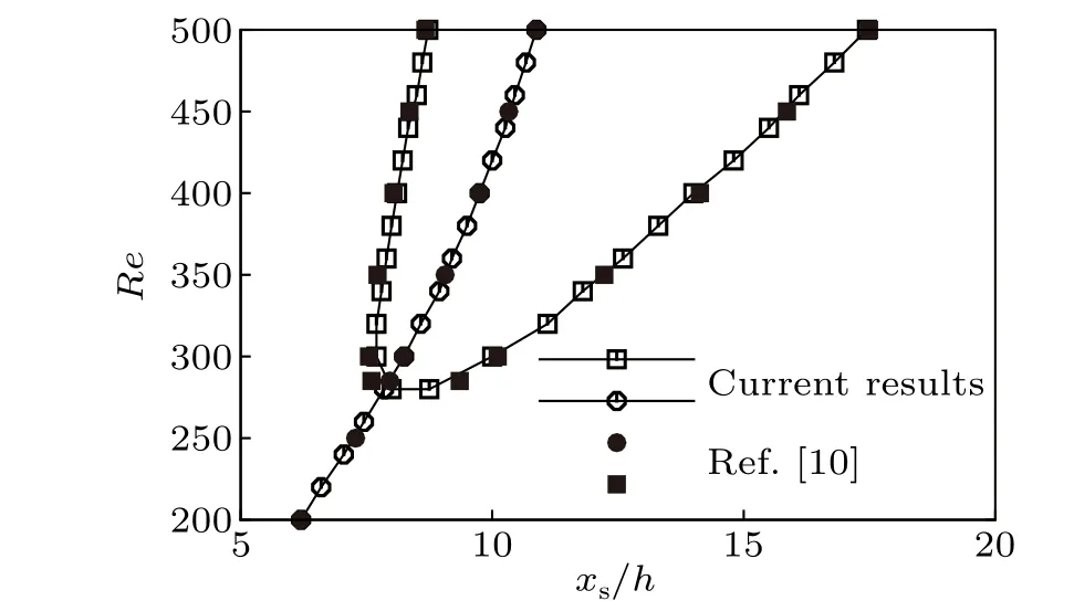
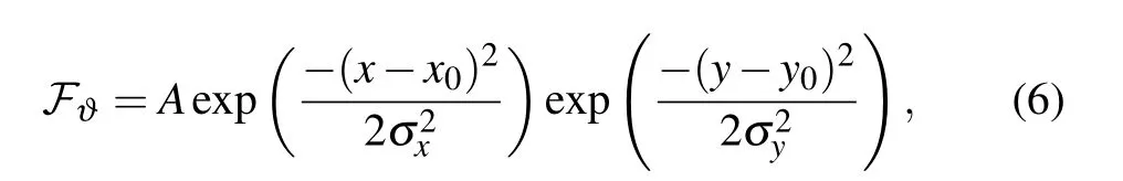
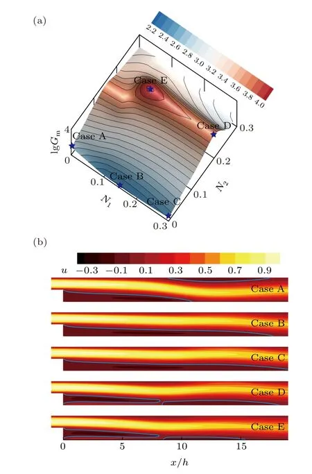
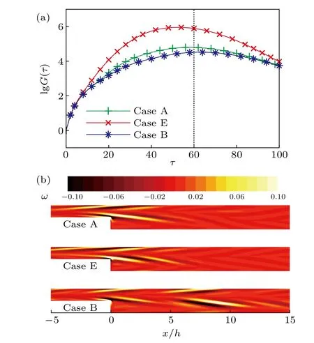
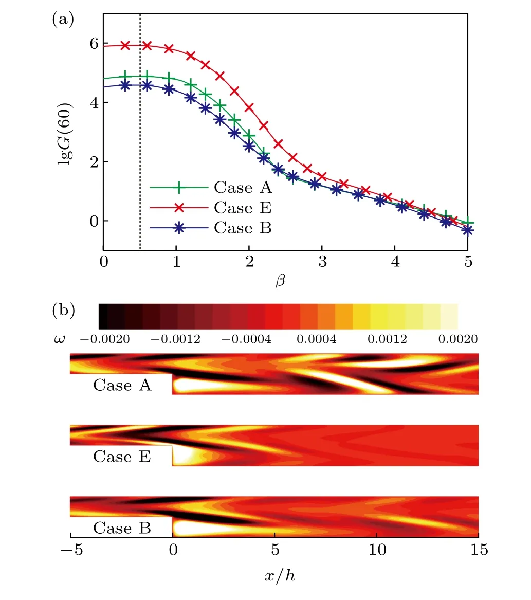
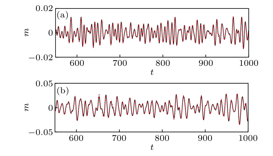
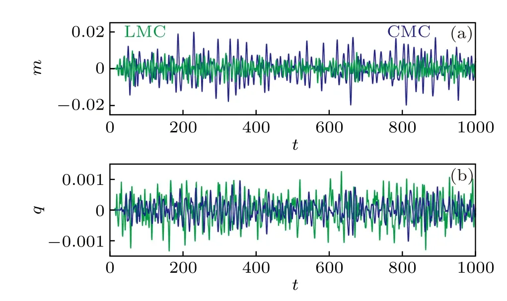
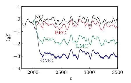
In BFC and CMC,the sphere of action is set as 0

3. Mesh and validation

All equations are solved with a high accuracy spectralelement method (SEM)[32]in the domain shown in Fig. 2.The spatial domain is split into 2039 quadrilateral finite elements, in which both the geometry and solution variables employ equal-order tensor-product Lagrange polynomial expansions. The flow separates near the corner of the step and the circumfluence in the separation bubbles generates near the upper and lower walls, so the grids there are refined. Gauss–Lobatto Legendre polynomials are adopted as a basis for the numerical solution. The time-stepping method based on the backwards-time differencing[33]is taken to perform the time integration. The Krylov subspace method and the Arnoldi decomposition method are employed to solve the eigenvalue in the optimal transient growth analysis.

Fig.2. Calculation domain and mesh.

Fig. 3. Separation bubble length varying with the Reynolds numbers from references and current results.

For the base flow solution, a Dirichlet condition is set atΓ∞(U=4y −4y2,V=0), and a Neumann condition is set atΓo(∇nU=0,∇nV=0). A no-slip Dirichlet condition is set atΓb(U=0,V=0). A high-order Neumann condition for the normal component along the boundary calculated from Eq.(1)is set for the pressure at all boundaries exceptΓowhere the pressure is set to be zero. For the linear stability analysis,the boundary conditions are similar with those in the base flow solution, but the perturbation velocityu′is set to be zero atΓ∞andΓb. For the optimal transient growth analysis, perturbations at all boundaries are set to be zero. Besides, readers cloud learn more about the detailed solution procedure of the eigenproblem in the optimal transient growth analysis via the achievements of Barkleyet al.[33]In all calculations,the timestep is set as 0.001 with the second-order time integration and eighth-order polynomials. The lengths of the primary and secondary separation bubblesxsas a function of Reynolds number are shown in Fig.3. Both lengths increase with the Reynolds number,and our results are consistent with those in the reference.

4. Results and discussion

4.1. Effects of BFC

The maximum amplification ratesGmof the initial Gaussian perturbationϑas well as the corresponding steady base flow with BFC are reported in Fig. 4.N1andN2represent the control numbers of the streamwise Lorentz force from A1and A2respectively.N1andN2constitute the coordinate system of control numbers. It is worth mentioning that the inlet noise source in BFC is also the noise sourceℱϑϑin LMC and CMC.In BFC,we mainly discuss the control effects based on the single initial wall-normalwise perturbation. In order to facilitate our research,it is assumed that the noise source obeys the Gaussian distribution,which could be written as

whereAis the amplitude of perturbations,(x0,y0)is the center of perturbations andσx,σyare the radiation radii of perturbations. The parameter in Eq. (6) are (x0,y0)=(−0.5,0.25),(σx,σy)=(0.1,0.1), andA=4.0, and the perturbation variableϑcould be expressed via the Dirac function.

It could be observed thatGmcould achieve the peak value at (0.1,0.2) while the minimal one at (0.15,0) according to Fig. 4(a). Meanwhile, the distributions ofGmalso illustrate that the streamwise Lorentz force only acting on SSB could reduce the maximum amplification rate, while acting on both PSB and SSB could achieve the opposite effects. In other words, it could stabilize the liquid metal flow via fixing SEA only in SSB, or destabilize the flow by setting SEA in both separation bubbles. Figure 4(b)demonstrates the steady base flows of which the maximum amplification rates are marked in Fig.4(a). Cases A–E correspond to the control numbers at(N1,N2)=(0,0), (0.15,0), (0.3,0), (0.3,0.2), and (0.1,0.2)respectively.The contour in Fig.4(b)is colored by the streamwise velocity. The solid blue lines represent the isolines ofU=0,and the liquid metal inside the isoline contains a backflow. Moreover,the isolines also present the scales of the separation bubbles. We can clearly see the PSB and SSB for the no-control (NC) case (case A). For case B, there only exists the PSB but its length is larger than that for case A because the streamwise Lorentz force could reduce the magnitude of the backflow velocity of the separation bubble, and then the bubble dwindles gradually. The decrease of SSB size may flatten the concave streamline near SSB, and then the separation streamline near PSB may lift up. Once the control strength from A1increases(case C),the length of PSB might take a growth. If the electromagnetic actuator A2is turned on, the PSB could be divided into two smaller bubbles (case D). However, the scale of PSB in the wall-normalwise direction is much larger than that of SSB,so effects of the streamwise Lorentz force on SSB size are more remarkable. It could be observed that the scale of the downstream divided bubble might be reduced once the control strength from A2decreases by comparing cases D and E.It is obvious that the amplification rate of the initial Gaussian perturbation energy is minimal for case B and maximum for case E.

Fig. 4. The maximum growth rates of the initial Gaussian perturbation for different control numbers and corresponding base flows. (a)The maximum growth rates. (b)The corresponding base flow.

Figure 5 shows the energy derivative varying with the time calculated from the Reynolds–Orr equation.[34]The energy derivative is nondimensionalized byE0/t0whereE0is the initial perturbation energy andt0is the unit time. Actually,dE/dthas a positive correlation to the rates of the curves in Fig. 4, andG(t)in Fig.4 achieves the peak value at the time corresponding to dE/dt=0 in Fig.5.

Fig.5. Growth rate of perturbation energy varying with the evolution time.

Figure 6(a) shows the optimal energy growth of perturbations over a given time intervalτ. It is the fact that the peak amplification rate of the perturbation energy in the optimal transient growth is much larger than that of the single initial Gaussian perturbation. We know that the optimal initial perturbations in the optimal transient growth are different and they are dependent on the time interval. It could be found that the optimal amplification rate of the two-dimensional perturbation always increases with the evolution interval and reaches to the peak value at aboutτ=60,and then decays.Figure 6(b)presents the optimal initial perturbations of which the optimal amplification rates atτ=60 are shown in Fig.6(a). The perturbation energies are normalized, and the contours are colored with the perturbation vorticity of the level from−0.1 to 0.1. The patterns of the optimal initial perturbations resemble the KH vortices,and always distribute along the separation line.The typical spatial distribution like the KH vortices in the optimal initial perturbation could diminish the effects of distortion and dissipation from the mean strain field because each initial perturbation could evolve into the KH-like vortices.

Figure 7 illustrate the optimal amplification rates of the three-dimensional perturbations for the evolution interval ofτ=60 and corresponding optimal initial perturbations. The optimal amplification rate of the three-dimensional perturbation energy slightly increases at small spanwise wavenumbers,and then decreases. The maximum value approximately appears atβ=0.5. The magnitude of the optimal amplification rate in case E is still the maximum one while that in case B is always the minimal one for the same spanwise wavenumber. This phenomenon indicates that BFC assurely increase or decrease the amplification rate of the perturbation energy in the liquid metal BFS flow. The three-dimensional optimal initial perturbation is visualized via the spanwise velocity. The distributions of the three-dimensional optimal initial perturbations are different from the two-dimensional ones. Besides the step corner and the outlines of the separation bubbles, most spanwise perturbations locate near the step. This distribution features are similar with those in Ref.[10].

Fig.6. The optimal amplification rate of two-dimensional perturbations and corresponding initial perturbations. (a)Optimal amplification rates varying with the evolution intervals;(b)corresponding initial perturbations.

Fig.7. The optimal amplification rate of three-dimensional perturbations and corresponding initial perturbations. (a) Optimal amplification rates varying with the spanwise wave numbers; (b) corresponding initial perturbations.

4.2. System identification in LMC and CMC

The above discussions have indicated that BFC could capably modify the perturbation energy in the liquid metal BFS flow. However, the flow system needs to keep laminar sometimes since the liquid metal contains a high heat transfer efficiency. The perturbation energy also could be amplified in BFC,thereby LMC and CMC are adopted to suppress the amplification of the perturbation energy in our control strategies.Certainly, CMC also could be employed to increase the perturbation energy because it contains BFC.It is noteworthy that LMC and CMC are performed based on cases A and B respectively. For contrast,the spatial distribution of the noise sourceϑin LMC and CMC is same with that in BFC,and the Lorentz force from the actuator A3also has the Gaussian distributions,and the parameters ofℱqfrom A3are(x0,y0)=(−0.05,0.01),(σx,σy)=(0.01,0.1), andA=4.0. Meanwhile, the perturbation variableϑcould be expressed as the Gaussian white noise with the standard deviation of 0.01 and the control inputqcould be written as the binary random function with the maximum amplitude of 0.0054 like Ref.[10].

Usually, referred to Ref. [31], the sensor S1is located downstream the noise source but upstream the actuator A3,and the sensor S2is placed near the reattachment point of PSB,thereby the signals of input and output in LMC and CMC are defined as follows:

Figure 8(a) shows the amplitude-frequency characteristics of the original input and output signals in CMC.In order to reflect the amplification features of the flow system on the noise,the signalssandmhere are obtained without the control input signalq. It can be seen that the amplitude of all signals attenuates rapidly when the frequency is greater than 1,so the low-pass filter could be adopted to extract the main parts of signals. The principle of the low-pass filtering is keeping the low-frequency amplitude-frequency characteristics as well as the amplitude of the original input and output signals. The transfer function of the low-pass filtering here is referred to Ref.[31]and could be written as

withη=0.8 andωc=2. Figure 8(b) shows the amplitudefrequency characteristics of the low-pass filtered signal. It can be seen that the filtered signals has the similar amplitudefrequency characteristics with the original signals. In addition, the amplitude–frequency characteristics of the original and low-pass filtered signals with the same transfer function in LMC also resemble those in Fig.8.

Fig.8. Amplitude–frequency characteristics of original and filtered signals.(a)Original signal;(b)filtered signal.

Although the amount of data in the control model needs to be reduced, it is still necessary to ensure that the sampling data is sufficient. As mentioned above,the time step is 0.001 in all calculations,so the sampling period is set to 0.1.Figure 9 shows the auto-correlation and cross-correlation functions between the sampling signals. Observing the auto-correlation function curve of the output signalm, it could be seen that the curve reaches the minimum value at the time oft=4.1 andt=6.0 for LMC and CMC respectively. That is to say,there might be a duration of 4.1 and 6.0 for the previous outputs having an impact on the subsequent outputs. Hence, the value ofnain the ARMAX models for LMC and CMC are 4.1/0.1=41 and 6.0/0.1=60 respectively. In addition, the cross-correlation function curves ofsandm,q,andmbegin to fluctuate intensely att=11.5 for LMC andt=22.5 for CMC.This phenomenon demonstrates the response delay time of the output to a single input is 11.5 and 22.5 for LMC and CMC respectively,so the values ofndsandndqin the ARMAX model should be around 115 for LMC and 225 for CMC. Once the cross-correlation function curves(green one)ofqandmtake an intense fluctuation,the time intervals between the first wave valley and wave peak are 2.9 and 4.2 for LMC and CMC respectively. This appearance indicates that the time interval of the input signal affecting the current output is 2.9 for LMC and 4.2 for CMC. Thereby, the value ofnbqin the ARMAX model is around 29 for LMC and 42 for CMC.In fact,as S1is close to A3, the value ofnbqis similar with that ofnbsin the ARMAX model.

Fig.9.Auto-correlation and cross-correlation characteristics of the measured variables. (a)LMC;(b)CMC.

The parameters in the ARMAX models for LMC and CMC are shown in Table 1. The primary sharp of signals predicted by the ARMAX model are mostly dependent on these parameters.na,nbq,nbs,ndq, andndsare usually determined fristly and thenncis adjusted to improve the goodness of fti between the predicted and sampling signals. The goodness of fti could be expressed as

wherempis the signal predicted by the ARMAX model andmris the sampling signal.Figure 10 shows the predicted and sampling signals. It could be observed that the output signals from the ARMAX model coincide with the sampling signals. The goodness of the fit is 91.2% and 86.4% for LMC and CMC respectively.

Table 1. Parameters in the ARMAX model.

Fig.10. The signals predicted by the ARMAX model(black line)and the sampling signals(red line).(a)Signals in LMC.(b)Signals in CMC.

Fig.11. The characteristics of impulse response in the ARMAX model.

Figure 11 shows the impulse response of the output signal to a single input signal in the ARMAX model. As discussed above, the start time of response has been shown in Table 1. For LMC,the amplitude of the response signal tends to 0 whent>35, while it still has slight fluctuations whent>65 and tends to 0 untilt>110 for CMC.It could be found that the two response signals for each control strategy fluctuate in opposite directions. The time for the output response to the noise signal achieving the peak value slightly lags behind the response to the control input signal,because the actuator A3is downstream the sensor S1. Comparing the maximum amplitudes of the response signals, we could observe that the peak amplitude of the response to the noise signal is greater than that of the response to the control input signal both for LMC and CMC, because the spatial distribution area of the noise source signal is larger than that of the control input signal.

4.3. Closed-loop control in LMC and CMC

Once the parameters of the ARMAX model are achieved,the transfer functions ofq →mands →mare identified. The coefficients in the transfer function are referred as the Markov parameters, which represent the impulse response of the system. If we want to know the future control signal according to the measured signal,the corresponding compensator needs to be designed to build a complete closed-loop system. The system without compensator is called an open-loop system. The relationship between the future output signalMT,the known(or measured) noise signalSg, the control signalQgand the future unknown control signalQfcould be constructed via the Markov matricesZs,Zq,andLqin any sampling time periodT. The expression could be written as

They could be achieved from the corresponding impulse responses in the ARMAX model. In Fig. 11, the impulse response of the output signal to the two input signals tends to 0 whent>35 for LMC andt>110 for CMC,so the time periodTshould be greater than 400 for LMC and 1100 for CMC in Eq.(10). If we want to get the control input signalQfin the next period,we must know the future output signalMTwhich is also the expected output signal. The control targets of LMC and CMC are completely suppressing the noise,that is to say‖MT‖22=0,thusQfcould be written as

HereL+qis the pseudo-inverse of matrixLqbecause matrixLqdoes not have an inverse matrix. Equation (12) defines a linear dynamic system where the input is the noise and control signal in the previous period,and the output is the control signal in the next period, so the compensator is also called a feed-forward controller. In the pseudo-inverse solution, the tolerance value needs to be set. The principle of tolerance setting is that the reciprocal of all singular values of the matrixLqare greater than the tolerance value. However, the amplitude of the impulse response of the output signal to the input noise signal in the compensator increases as the tolerance decreases.In other words,growth of the amplitude of the control signal might improve the control cost. If the tolerance value is not considered,the performance of the compensator could be better for a longer time period. Meanwhile,it could take more time to completely suppress the noise. The tolerance value is set to 0.15 for both LMC and CMC,and the time period is set tot=100 andt=180 for LMC and CMC respectively.

Figure 12(a) shows the impulse response of the output signal to the noise signal for the close-loop and open-loop systems. The dashed line represents the open-loop system, and the solid line represents the closed-loop system. Compared with the output signal without the controller,the response amplitude of the output signal decreases significantly after applying the controller, and tends to 0. Figure 12(b) shows the impulse response of the output signal with the controller to the noise signal, which is also the required control input signal for the closed-loop system. It can be seen that the control input signal decreases rapidly from the maximum value at the beginning, and then exhibits a damped oscillation and finally decays to 0.

Fig. 12. The impulse response of output to input in LMC and CMC.(a)Impulse response of m to s;(b)impulse response of q to s.

Fig.13.Outputs of the open-loop system and close-loop system in LMC and CMC.(a)Open-loop system;(b)close-loop system.

Fig.14. Control inputs of the close-loop system.

Figure 13 shows the output signals obtained in the openloop and close-loop systems. The signals in Fig. 13(a) from the open-loop system are the original filtered signals. The amplitude of the signal for LMC is less than that for CMC because the the location of S2for CMC is downstream that for LMC.Although the peak amplification rate for case B is much less that for case A, the measurements in local regions still grow along the flow direction. It can be seen that the pulsation amplitude of the output signal is reduced by 86.5%and 95.3%for LMC and CMC respectively after applying the controller.

4.4. Comparison

Figure 15 shows the perturbation energyℰ=∫Ω0.5(u′2+v′2)dVof the entire liquid metal flow system varying with the evolution time for different control strategies. The black line, red line, green line and blue line represent the perturbation energy for NC, BFC, LMC and CMC respectively. All controls are turned on att= 2000. We could find that the magnitude of the perturbation energy in the liquid metal flow could be reduced once the electromagnetic actuators are turned on. The average value of the perturbation energy in the time period oft=2500–3500 is reduced by 54.9%, 97.4%, and 99.8% for BFC, LMC and CMC respectively. We could observe the profiles of NC and LMC have some overlap parts at beginning, and this phenomenon also exists for BFC and CMC.As discussed above,there exists a time interval for the response of the output signal to the input signal. We know the control targets of LMC and CMC are completely suppressing the noise,but the perturbation energy could not be suppressed completely. However, the magnitude of the perturbation energy could be reduced by 2 orders in LMC, and 3 orders in CMC.The inherent properties of amplification are responsible for this phenomenon. The sensor S2just could measure the local perturbation energy,and perturbations in other parts also be amplified. BFC could change the amplification features of the liquid metal BFS flow,and the linear control model could reduce the magnitude of the perturbation energy of whole liquid metal BFS flow. At least, CMC could achieve a better suppression of the perturbation energy compared with BFC and LMC.Since CMC is the combination of BFC and LMC,we could adjust the instability in the liquid metal BFS flow by turning on or turning off some actuators.

Fig.15. Variations of the perturbation energy of the whole system for different control strategies.

5. Conclusion

To summarize, TEA and SEA could be applied to adjust the perturbation energy in the liquid metal BFS flow. Setting SEA in both PSB and SSB could amplify the magnitude of the perturbation energy, while combination of TEA, SEA (only acting on SSB)and two sensors could suppress the amplification of the perturbation energy. These results manifest that the electromagnetic actuators have the satisfied regulation effects on the perturbation energy in the liquid metal BFS flow, and the strategy of CMC could be commendably applied to engineering.

Acknowledgment

Project supported by the National Natural Science Foundation of China(Grant No.U2141246).