QU Bo , and SUN Wenjing

1) School of Science, Nantong University, Nantong 226007, China

2) YK Pao School, Middle School Campus, Shanghai 200336, China

Abstract Biogenetic sulfide dimethylsulfide (DMS)plays a major role on the global climate, especially in Arctic Ocean. Accurate simulate DMS concentration is an important task. Here we introduced both biogeochemical depth-averaged model G93 and its extension model-one dimensional DMS model. Both surface concentrations, vertical profiles of chlorophyll (CHL)and DMS are simulated using the two models within southern Greenland Sea (0˚E – 10˚E, 70˚N – 75˚N)during year 2012. As the input data for the models simulations, the spatial monthly mean of methodology forcings including sea surface temperature (SST), wind speed (WIND), cloud cover (CLD), sea ice concentration (ICE)and mixed layer depth (MLD)are calculated. Satellite 8-day time series of chlorophyll-a(CHL)are used as observation data for CHL related parameter calibrations. Simó’s imperial formula is used as the monthly DMS observation data. The Genetic Algorithm technique is used for the parameter calibrations. The simulation results show that the most DMS related surface concentrations exhibit the normal distributions with peak during May. CHL, DMS and DMSP (dimethylsulphoniopropionate)vertical profiles are obtained for July, August and September in year 2012. CHL had the higher variation of subsurface concentration maximum (SCM)in July with the lower surface concentration value. DMS had surface higher and subsurface lower profile for the all three months. DMSP also had subsurface high in July. The SCM CHL diurnal variation in the subsurface also can be resulted from diurnal changes in MLD and vertical mixing variations, plus photolysis and wind-driven ventilations.

Key words dimethylsulfide; vertical profile; chlorophyll; biogeochemical modeling; Greenland Sea

1 Introduction

Dimethylsulfide (DMS)is an important sulfur gas from ocean to the atmosphere. It comprises nearly 60% of the global biogenic sulfur emission to the atmosphere (Bateset al., 1992). DMS marine emission could be a precursor of tropospheric aerosols and could form cloud condensation nuclei (CCN)in the remote marine atmosphere,hence affect the earth radiative balance and thus cool the climate (Charlsonet al., 1987; Kiene and Bates, 1990).The initial increases in DMS were because of the decomposition of its biogenic precursor dimethylsulphoniopropionate (DMSP), while DMSP is synthesized in the cells of phytoplankton species (Andreae and Barnard,1984; Kelleret al., 1989). Climate controls on the phytoplankton (we use chlorophyll to represent)through physical factors such as SST, light and nutrient regimes and mixed layer depth (Quet al., 2006). The process of DMS formation and its reaction to the climate is a complex process and many issues are unresolved.

The most effective region of DMS emissions to the climate is polar region (Levasseur, 2013). Many researches focused on the surface chlorophyll concentrations and surface DMS mass concentrations to estimate the amount of DMS sea-to-air flux, in order to measure how much effect of DMS emission to the climate (Daviset al.,1998; Gabricet al., 1998, 2003, 2005; Chalecki, 2007;Matrai, 2007; Galí and Simó, 2010; Qu and Gabric, 2010;Humphrieset al., 2012; Trevena, 2012; Ghahremaninezhadet al., 2016; Quet al., 2016, 2017, 2021a; Ghahremaninezhadet al., 2019). The vertical DMS simulations are lacking, except a few early researches (Olliet al.,2002; Croppet al., 2004; Gabricet al., 2008; Lundénet al., 2010; Liuet al., 2012; Ghahremaninezhadet al.,2017). Comparing to horizontal advection, the vertical physical dynamics of the mixed layer are crucial driving forces in shaping regional ecosystem dynamics (Croppet al., 2004). The interaction of light penetration and the mixed layer depth together with the supply of nutrient into the mixed layer are important limiting factors on biological production (Andreae and Barnard, 1984; Kelleret al., 1989; Doneyet al., 1996).

Subsurface chlorophyll (CHL)is also neglected during most of researches. Cherkashevaet al. (2013)indicated that overall monthly surface CHL profiles in the Greenland Sea had highest surface CHL values in April and lowest in July to August. Low surface CHL are usually an indication of subsurface CHL maximum. The maximum CHL concentrations started in the great depth in the spring and gradually moved towards surface in September(Cherkashevaet al., 2013).

In this paper, we introduce a depth-averaged biogeochemical model (G93)using the most realistic parameter set to calculate regional surface DMS concentrations (Gabricet al., 1993, 1999). Genetic algorithm technique is used for the model parameter calibretions based on satellite CHL time series and DMS observation data which was calculated using the empirical formula of Simó and Dachs (2002). Using those calibrated parameters, a onedimensional model is obtained from the depth-averaged G93 model by resolving the distribution of concentrations and fluxes over depth in the water column and allowing diffusive and advective fluxes (Croppet al., 2004; Gabricet al., 2008). We then calculated the vertical profile of DMS for July, August and September of year 2012. Compared our results with the observed data from Ocean University of China and calculated data from empirical formula (Simó and Dachs, 2002). The vertical profile of DMS using our 1-D model is calculated which is quite close to the field data and calculated data (Croppet al.,2004).

2 Data and Model Structure

2.1 Data Sources

Our study region is restricted within southern side of Greenland Sea (0˚ – 10˚E, 70˚ – 75˚N)(Fig.1). The time series of surface CHL and DMS for year 2003 to 2020 are retrieved from the Giovanni online retrieval system(https://giovanni.gsfc.nasa.gov/giovanni), developed and maintained by the NASA GES DISC (Acker and Leptoukh, 2007). Based on the field data obtained by Ocean University of China (OUC)in Greenland Sea and Norwegian Sea (Liet al., 2015), the time period of July to September in year 2012 is chosen for vertical DMS related profile calculations and comparisons. The forcing for 2012 for the depth averaged G93 model calibration and calculation are obtained from the following sources: the 8-day CHL time series for year 2012 is retrieved from the satellite data within MODISA (Aqua), Level-3, 8-day, mapped archive (https://oceancolor.gsfc.nasa.gov/). Weekly ICE for year 2012 is obtained from the database at http://iridl.ldeo.columbia.edu/SOURCES/.NOAA/.NCEP/.EMC/.C MB/.GLOBAL/.Reyn_SmithOIv2/. Weekly SST and surface wind speed for year 2012 were retrieved from the Remote Sensing Systems (RSS)archive at http://www.remss.com/.

Fig.1 Study region (red box)and its surroundings, together with the surface flow direction vectors.

CLD in year 2012 is calculated from the NASA archive available at http://gdata1.sci.gsfc.nasa.gov/daac-bin/G3.The conductivity temperature and depth (CTD)data is used to calculate mean MLD in year 2012 (using 0.5℃lower than surface temperature as criterion), where CTD data is obtained from the Arctic Ocean measurement database (https://catalog.data.gov/dataset).

2.2 Depth-Averaged Model and Calibration Method

2.2.1 G93 model

A biogeochemical model-G93 (Gabricet al., 1993,1999)is used to simulate regional DMS concentrations.The G93 model was originally proposed by Gabricet al.(1993)and later extended to include seasonal light and temperature variations (Gabricet al., 1999). G93 model is essentially a nitrogen-based ecosystem model with unidirectional coupling to a sulfur-based biochemical model.The nitrogen and sulfur models are decoupled when analyzing the dynamics (Croppet al., 2004). G93 has been applied to polar regions (Gabricet al., 2004, 2005; Qu and Gabric, 2010; Quet al., 2016, 2017, 2021a). The model contains comprehensive food web system. The model averages over mixed layer and all parameter values are scaled by the depth of the mixed layer.

There are two main parts of the sub-models (Gabricet al.,1999; Qu and Gabric, 2010; Quet al., 2016, 2021b). First sub-model is the nitrogen-based PZN model and the second sub-model is the sulfur-based DMS model. The PZN sub-model includes some biological rate parameters,including the biomass of phytoplankton (P), the biomass of zooplankton (Z), the available nutrient concentration(N), and some more parameters describing a physical forcing on the phytoplankton growth rate (Quet al., 2016)(see Table 1). Wherekiare defined in Table 1.µis phytoplankton nitrate-specific growth rate, which has been parametrized using the formula:

Here,RN,RLandRTare the growth contemporaneously limited by nutrient availability, light and temperature respectively.µ0is the phytoplankton maximum growth rate.DMSPandDMSare the concentrations of DMSP and DMS respectively. The model is closed with respect to mass,N0=P+Z+N, so that the model biotic compartments do not eventually run out of nutrient. The model parameters and calibrated data are defined and listed in Table 1.

The model is calibrated using satellite data on CHL for the PNZ sub-model, and available DMS field data for the sulfur sub-model. We note that parameter calibration is difficult for the sulfur sub-model due to the limited set of DMS observations available for the Arctic Ocean. Calibration parameters are as follows: the six most sensitive parameters related to CHL arek4,k19,k20,k23,IkandN0(=P+Z+N); the five most sensitive parameters related to DMS arek27,k28,k29,k31and γ (see Eqs. (1)– (5)and Table 1).

Table 1 Parameter definition in the G93 model

Model key parameters are calibrated using a genetic algorithm (GA)optimization technique (Holland, 1975).GA uses a class of optimization procedure to find the optimal solutions to a given computational problem that maximizes or minimizes a particular function. By using evolutionary computation, GA can mimic the biological processes of reproduction and natural selection to solve for the ‘fittest’ solutions.

The monthly mean meteorological forcings for WIND,SST, CLD, ICE and MLD for year 2012 are supplied as a meteorological file input. GA calibrations are then carried out both for CHL and DMS related key parameters. The fitness function uses a chi-squared (χ2)statistic to minimize the difference between the observed data and model simulation data (Qu and Gabric, 2010; Quet al., 2016).

The 8-day mean satellite CHL data of year 2012 (from March to September)is used for CHL observation data.Monthly DMS concentration observation data is derived by using the empirical formula provided by Simó and Dachs (2002):

where the units ofMLDare meters,CHLare mg m-3, andDMSare nanomoles (nmol L-1).

After calibration, the biogeochemical model G93 is rerun using the calibrated parameter set and the horizontalDMSrelated output is obtained.

2.2.2 1-D DMS model

One-dimensional DMS model is further used for calculating vertical profiles of DMS. It uses the method of lines to solve the partial differential equations (Schiesser,1991). The finite difference approximation method is used for the spatial dimensional derivative calculations.Then it coupled with time-dependent ordinary differential equation at each grid point. A Runge-Kutta integrator is then used for efficiency advanced solution in time at each point in the water column. The accuracy and stability of the method are well controlled by the model itself (Schiesser, 1991).

HereC(z,t)is state-variable concentration.kvis the vertical advection velocity (m d-1). The vertical turbulent diffusivityD(z,t)(m2d-1)is calculated in a separated off-line computation (Bailey, 2008).G(z,t)is net production which represents the difference between the production and loss terms. For each state variable,G(z,t)is replaced by the right hand side of equations in G93 model(Quet al., 2016). Because in 1-D model, DMS sea-to-air emission as a boundary condition, the effect of zooplankton feeding disturbances on DMS is not yet clear. Hence,the model does not take into account the vertical movement of zooplankton. Similarly, the effect caused by sedimentation of DMS is insignificant compared to the DMS sea-to-air flux, and is therefore ignored in the model.

Because light intensity varies at different depths, the rate of growth of specific phytoplankton in this one-dimensional model also varies with depth. Eq. (1)is also valid in 1-D model. The relationship is described by Walshet al. (2001)as follows:

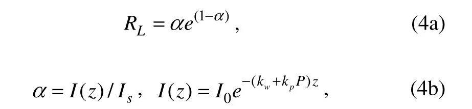
wherekwis the light attenuation of seawater,kpis the light attenuation because of phytoplankton self-shading.zis the depth (unit is meter),I0andIsare the incident surface irradiation (W m-2)and the phytoplankton saturating irradiation (W m-2)respectively.

The temperature dependence of phytoplankton growth is as follow (Eppley, 1972):

Here,Tis for temperature (℃)andTmaxis the maximum annual temperature.Tmay vary with depth. In general, when the depth of thermocline and density hops are similar, the temperature of the ocean mixing layer is more consistent.

Availability of nutrientRNis defined as follow:

Hereksis the nitrate half-saturation concentration.

According to Gabric Parslow (1989), the boundary condition of 1-D model (Eq. (3))is given by

ξis a parameter specifying the nature of the boundary.Whenkvis non-zero, ifξ= 1, a perfect absorbing boundary is specified; ifξ= 0, a perfect reflecting boundary is specified.

The sea-to-air DMS flux is calculated as the production of transfer velocity and DMS concentration, where the atmospheric concentration of DMS is neglected according to Liss and Merlivat (1986). The transfer velocitykwis calculated in terms of wind speed cm h-1)(at 10 m above surface)and SST in ℃ using the empirical formula of Nightingale (2000)(Gabricet al., 2008).

An S-function is used to generate diffusivity profile during model simulation (Croppet al., 2004):

HereDis the diffusivity with unit of m2d-1.DmaxandDminare the maximum mixed layer diffusivity and minimum sub-mixed layer diffusivity.zis the depth of the water column (m). The depth of the model domain isH(meter). MLD is mixed layer depth (m).ris a parameter that controls the steepness of the pycnocline (1

A similar function (9)is also used in the model to describe the vertical temperature profile, where the temperature (Tmax)in the mixing layer is also assumed to be uniform, and the temperature (Tmin)in the sub-mixed layer is represented by a fixed value, as shown below:

An important parameter in the vertical model is the diffusivityD(also called diffusion coefficient)in Eq. (12).Diffusion coefficient is a measure of diffusion ‘rate’,which is very important for the quantitative treatment of diffusion. There have been many laboratory studies on determining diffusion coefficients, and some typical diffusion coefficients have been obtained. When a system is randomly disturbed, the diffusion coefficient is much larger than in the absence of disturbance. In our study, the movement of zooplankton, phytoplankton, wind speed,SST, and ice sheet disturbances all have a significant impact on the determination of diffusion coefficients.

Horizontal diffusion has less impact on mixed-layer ecosystems than vertical diffusion, so we ignore the effects of horizontal stratospherics and consider only vertical diffusion in seawater (Croppet al., 2004). The vertical vortex diffusion coefficient in seawater is usually 10-5m2s-1(Zhang, 2008). In general, diffusion in the Arctic Ocean is weak, so the corresponding diffusion coefficient is also smaller, ranging from 10-6m2s-1to 10-5m2s-1. In this study, constants 10-5m2s-1and 10-6m2s-1were used as the initial upper and lower limits of the diffusion coefficient, and on this basis, approximate diffusion coefficient data were obtained according to the Eq. (8).

3 Results

3.1 Forcings of Methodology Data

Monthly mean SST, WIND, ICE, CLD and MLD is plotted in Fig.2. Mean SST is within 1.0℃– 5.7℃ with peak month in August; CLD is in the range of 82.2% –93.3%; Mean wind speed is higher in winter and lower in summer, with range of 5.32 – 13.2 m s-1; ICE is within 2.12% – 25.85% in the southern GS; and MLD is higher in winter and lower in summer, with the range of 12.4 m to 266.78 m. The much deeper MLD occurred during January to April, over 200 m.

Fig.2 Monthly mean forcings for year 2012 in the study region.

3.2 GA Calibrations and the Regional Output

For using biogeochemical model G93 to calculate the regional DMS, genetic algorithm (GA)calibration for CHL related key parameters (k4,k19,k20,k23,IkandNo(=P+Z+N))are done first. The observation data is 8-day mean CHL time series from MODIS satellite data. The total nutrient value ‘N0’ was set to a few hundreds, in order to generate a spring bloom (Gabricet al., 2005; Qu,and Gabric, 2010; Quet al., 2016). The model simulation results are compared with the MODIS satellite 8-day mean CHL time series (Fig.3a). Notice that the horizontal axis started from day 88 and finished at day 272. The peaks are not matched well, but this is the best results we can get. The basic pattern is matched between model simulated result and MODIS satellite data. The fitness function is used for tuning the difference between the model and MODIS data using the time square root (χ2)function. The more close to zero (fitness function value),the more accurate the simulation is.

Fig.3 GA calibration results for (a)CHL and compared with MODIS satellite CHL data; (b)DMS and compared with the DMS calculated data according to the imperial formula of Simó and Dachs (2002).

DMS related key parameters (k27,k28,k29,k31andγ)are calibrated afterwards in the similar method (Fig.3b). The observation DMS data is monthly data based on the imperial formula of Simó and Dachs (2002)according to the satellite monthly CHL and monthly MLD of regional forcings. The calibrated parameters are shown in the figures.

The model outputs for DMSP, Z and DMS flux (are shown in Figs.4a and 4b). The peak of DMS, DMSP and zooplankton are all in day 168, 8 days after peak of CHL.The peak of DIN is in day 200, the time when DMS,DMSP and Z had a dip at this time. There are negative correlations between DIN and DMS related parameters during the period of day 168 to day 256. With the decrease(increase)of DIN, DMS related parameters increase (decreases). The peak DMS flux occurs at day 156, 8 d before the peak of DMS (Fig.4b).

Fig.4 G93 simulation output for (a)CHL, DMS, DMSP, Z and DIN; (b)DMS flux and DMS in the study region.

3.3 Vertical Profile of CHL, DMS and DMSP

The input data of the 1-D model in this paper includes SST, WIND, photosynthetically active radiation (PAR),MLD, and diffusivityD, where weekly data of SST and WIND are used in the model. PAR uses 8-days data, and MLD uses monthly data. Based on the G93 model calibration results, the 1-D vertical model is simulated and the vertical distributions of CHL, DMS and DMSP are obtained within the depth of 60 m in July, August and September of 2012 in the southern region of the Greenland Sea (0˚ – 10˚E , 70˚ – 75˚N).

During the simulation process, with a depth interval of 2 m and a total of 31 data points of 60 m are used. For July and August data, it has grid of 31× 31 matrices, and September data has grid of 31× 30 matrices. Basically, the average CHL, DMS and DMSP concentrations at each depth are calculated for the three selected months, and the vertical distributions in July (solid blue), August (dash green)and September (dash red)are drawn using MATLAB program, as shown in Fig.5.

CHL had smaller CHL surface concentration (< 0.94 mg m-3)in July and higher surface concentration in August and even higher surface concentration in September.According previous surfaceCHLconcentration simulations, the peak ofCHLshould be in April or early May.CHLstarted to drop after June and the second peak should occur in September. This is correct surface CHL concentration order. For lower surfaceCHLin July, the subsurface peak occurred between depth of 30 m – 40 m(Fig.5a). For the August CHL profile, there is less significant of subsurface peak (between 35 and 50 m depth).CHLreduces significantly below 50 m. In September, for the second surface peak, there is almost no subsurface peak. SurfaceCHLreaches the highest in September.There is a decreased trend underneath 40 m.

Fig.5 Vertical profile of (a)CHL; (b)DMS; (c)DMSP, in July, August and September of 2012 in the study region.

DMS vertical concentration (Fig.5b)shows the surface DMS was higher in August and lower in September.There is no subsurface peak for DMS profile. DMS concentration reduces significantly below surface of 30 m for July and August. However, for September, DMS profile reduces gradually underneath the surface water.

DMSP vertical profiles are differently from DMS’s(Fig.5c). DMSP had smaller surface concentration in July,but had subsurface peak below 30 m. Slightly higher surface DMSP concentration in August had less significant subsurface peak (between 35 and 50 m). The concentration reduced sharply below 50 m. The September surface peak of DMSP had no subsurface peak and reduced concentration below 40 m.

3.4 Validation of the 1-D Model

Croppet al. (2004)and Gabricet al. (2003)have compared the one-dimensional DMS model (Eq. (8))simulation results with Eqs. (2a)and (2b)from the empirical formula by Simó and Dachs (2002). Their results revealed that the DMS simulated by the one-dimensional DMS model are very closely correlated with the calculation results from the formula by Simó and Dachs (2002).Croppet al. (2004)also compared model results with the BATS data (Bermuda Atlantic Time-series Study)(http://bats.bios.edu/bats-data/)and found that the model does a good job of reproducing the major characteristics of the BATS data; however, does not do a good job of reproducing the fine detail, due to the 1-D model uses a homogeneous mixed layer and does not resolve the fine details of DMS concentrations.

The field data of DMS in the similar study region along depth provided by Liet al. (2015)(Fig.6a). The measureed DMS concentration from Liet al. (2015)is within 0.8 – 3.6 nmol L-1with average concentration of 2.82 nmol L-1(Fig.6a). Our simulated DMS concentration is within 1.18 – 2.26 nmol L-1with average of 1.96 nmol L-1. Considering the study region is not exactly the same, the depths are different. With 60 m in our simulation and 4000 m in the field data, the error is understandable.

Different from the result obtained by Gabricet al.(2008)when they did simulation in the Sargasso Sea during July - August 2004, the DMS subsurface diurnal variation occurred just 10 - 15 m below the surface waters.Our DMS profile had no diurnal variation in the DMS subsurface profile. The reasons are not clear. But it must relate to the different locations and different years with different mixing and stratification processes. If below the surface layer, much weaker mixing and attenuate light may allow the biochemical factors to create a peak of DMS profile underneath the mixed layer (Gabricet al.,2008).

The DMS surface concentrations simulated by 1-D model and by G93 model are also compared for July,August and September of 2012 (Fig.6b). The simulated DMS concentration using G93 is about 30% lower than 1-D model. The results using Simó’s emperial formula(Simó and Dachs, 2002)is over estimated in July and September (Fig.6b). The 30% error could be related to the accuracy problem caused by the large time interval between the input data, as well as lacking of accuracy of the diffusion coefficient calculation method. More accurate simulations are expected to carry out in the future.

Fig.6 (a)DMS concentration image observed by Li et al.(2015), where BB1, …, BB9 represent the stations in the study region; (b)DMS sea surface concentration comparison among 1-D model, G93 model and Simó’s imperial formula (Simó and Dachs, 2002).

4 Discussion

4.1 The role of MLD Related with DMS Production

Charlsonet al. (1987)have suggested that the plankton-climate interaction is self-regulated. Simó (1999)found that the MLD has substantial influence on DMS production in a short term. Researches indicated that vertical mixing affects phytoplankton as well as heterotrophic bacterial production by subjecting microorganisms to different degrees of exposure to ultraviolet (UV-B)and total solar radiation (Herndlet al., 1993; Somavillaet al.,2017). In shallower MLD, heterotrophic bacterial activity is more inhibited by UV-B and hence with less bacterial sulphur demand. In contrast, in deeper MLD, DNA (deoxyribonucleic acid)is easier to be repaired and recovered. Therefore, non-DMS-producer increases in the deeper mixed layer. DMS reduces underneath the surface water. Peak of DMS concentration appeared in the surface water. MinimumDMSappeared in the deep layer. Our simulation result (Fig.5b)agrees this result.

In our study region, diatoms dominated in spring (Zhanget al., 2014, 2017). Diatoms are the high phytoplankton producer and weak DMSP producer (Simó, 1999). This phenomenon caused higher CHL and lower DMS concentrations in spring. After the peak of CHL, CHL started to decrease, food-web changes accordingly. During strong stratified waters, phytoplankton biomass recycled via the microbial loop, thus facilitating a more rapid turnover of phytoplanktonic DMSP (Dacey, 1998). Hence, DMS production increases.

4.2 Subsurface CHL Maximum (SCM)

The subsurface CHL maximum (SCM)is likely associated with the supply of new nutrients from below the mixed layer (Boumanet al., 2020). It has been argued that satellite surface CHL concentrations may significantly underestimate water-column phytoplankton biomass in the Arctic Ocean (Martinet al., 2012). Changes in nutrient supply and light availability in water column may cause the SCM to increase to a great extend (Popovaet al., 2010).

Greenland Sea is one of the few areas in the world where deep convective mixing occurs and possible transferring great amount of carbon dioxide to rather deep layer (Reyet al., 2000). The rather complex hydrography and the sea ice drift provide special conditions for nutriaents, stratification and advection of sea ice (Cherkashevaet al., 2013). This causes the CHL vertical profile varies in different month and seasons. With strong vertical stratification and mixing in the mixing layer, plus ventilation and photo-oxidation losses in the surface layer during night, lower surface concentration appeared (Gabricet al.,2008).

Cherkashevaet al. (2013)did research on CHL vertical profile in Greenland Sea combining CHL cruise data for 1991 – 2010 and ARCSS-PP database for 1957 – 2010 and found that surface low value ofCHLare usually an indication of SCM. They also indicated that the contribution of SCM to the totalCHLin the case of low surface concentration can be important, with maximum SCMs exceeding surface CHL by up to a factor of three. This is true for our simulation results. With July surface CHL being the lowest, the SCM is the most significant and the increase of SCM is about a factor of one point six in our simulations (Fig.5a). In the results of Cherkashevaet al.(2013), the maximum of CHL vertical profiles gradually moved from great depths in spring towards surface in September. Our results also shows the similar trend from July to September (with the peak of CHL moved from underneath to the surface by September).

5 Conclusions

A depth averaged biogeochemical model G93 is introduced and calibrated according to the satellite CHL time series andin situdata of OUC in the southern Greenland Sea for year 2012. One dimensional vertical DMS model then introduced and simulated using calibrated parameters using G93 model as well as the input of SST, WIND,PAR, MLD, and diffusivity D. Genetic algorithm technique is used for model parameter calibrations. The most DMS related surface concentrations exhibit the normal distributions with peak during May. During July, August and September, vertical CHL, DMS and DMSP profiles are obtained by running 1-D vertical DMS model. CHL had the higher variation of SCM in July due to the lower surface concentration value. DMS had surface higher and subsurface lower profile for the all three months. DMSP also had subsurface high in July. The reason of CHL SCM could be due to the sea ice melting caused stratification during spring and summer and caused lacking of nutrients in the surface layer (Cherkashevaet al., 2013). The CHL diurnal variation in the subsurface also can be resulted from diurnal changes in MLD and vertical mixing variations, plus photolysis and wind-driven ventilations (Gabricet al., 2008). Recent research from Galíet al. (2019)pointed out that the reduction of sea-ice extend in Arctic Ocean is consistent with the increase trend of DMS oxidation production. In the future, Arctic waters is going to be more freshen due to the increase of ice melting with global warming trends. Coupling with the atmospheric circulation patterns would favour the sea ice advecting out of the Arctic Ocean, this will lead stronger water stratification. We can predict that low surface CHL and DMS with SCM may become even more frequently, because the nutrients will not reach to the top layer during melting season. More accurate vertical profile simulation is needed by improving the accuracy of the diffusivity calculations. More accurate DMS observation data is urged for more accurate parameter calibrations of the remote Arctic Ocean.

Acknowledgements

Sincere thanks should first go to Prof. Albert Gabric for his supervision of programming of 1-D vertical DMS model. Thanks to NASA Ocean Biology Processing Group and Goddard Space Flight Center of SeaWiFS Project Group for providing MODIS CHL data. Thanks to the Naval Research Laboratory Remote Sensing Division, the Naval Center for Space Technology, and the National Polar-orbiting Operational Environmental Satellite System (NPOESS)for providing WIND, SST data. We acknowledge Dr. David L. Carroll from CU Aerospace, for providing the genetic algorithm FORTRAN code.