Chunlei LIU, Yazhu YANG, Xiaoqing LIAO, Ning CAO*, Jimmy LIU, Niansen OU,Richard P. ALLAN, Liang JIN, Ni CHEN, and Rong ZHENG

1South China Sea Institute of Marine Meteorology, Guangdong Ocean University, Zhanjiang 524088, China

2CMA-GDOU Joint Laboratory for Marine Meteorology, Guangdong Ocean University, Zhanjiang 524088, China

3College of Ocean and Meteorology, Guangdong Ocean University, Zhanjiang 524088, China

4Department of Mathematics, Trinity College, University of Cambridge, Cambridge CB2 1TQ, UK

5Department of Meteorology, University of Reading, Reading RG6 6BB, UK

6National Centre for Earth Observation, Reading RG6 6BB, UK

ABSTRACT The change in ocean net surface heat flux plays an important role in the climate system. It is closely related to the ocean heat content change and ocean heat transport, particularly over the North Atlantic, where the ocean loses heat to the atmosphere, affecting the AMOC (Atlantic Meridional Overturning Circulation) variability and hence the global climate.However, the difference between simulated surface heat fluxes is still large due to poorly represented dynamical processes involving multiscale interactions in model simulations. In order to explain the discrepancy of the surface heat flux over the North Atlantic, datasets from nineteen AMIP6 and eight highresSST-present climate model simulations are analyzed and compared with the DEEPC (Diagnosing Earth's Energy Pathways in the Climate system) product. As an indirect check of the ocean surface heat flux, the oceanic heat transport inferred from the combination of the ocean surface heat flux, sea ice,and ocean heat content tendency is compared with the RAPID (Rapid Climate Change-Meridional Overturning Circulation and Heat flux array) observations at 26°N in the Atlantic. The AMIP6 simulations show lower inferred heat transport due to less heat loss to the atmosphere. The heat loss from the AMIP6 ensemble mean north of 26°N in the Atlantic is about 10 W m-2 less than DEEPC, and the heat transport is about 0.30 PW (1 PW = 1015 W) lower than RAPID and DEEPC. The model horizontal resolution effect on the discrepancy is also investigated. Results show that by increasing the resolution,both surface heat flux north of 26°N and heat transport at 26°N in the Atlantic can be improved.

Key words:ocean net surface heat flux, ocean heat transport, discrepancy, simulations, observations

1.Introduction

The ocean net surface heat flux (FS) determines how much energy enters the ocean. It is an indicator of the Earth’s energy budget imbalance, since about 84%-93% of the excess energy entering the Earth system has accumulated in the ocean (Von Schuckmann et al., 2016, 2020; Cheng et al.,2017; Cuesta-Valero et al., 2021), due to the small heat capacity of the atmosphere and upper layer soil. Regionally,FSis also closely related to the oceanic heat transport, which affects regional climates (Caesar et al., 2021) and the intertropical convergence zone (Frierson and Hwang, 2012;Donohoe et al., 2013; Kang et al., 2018). Therefore, accurate estimation ofFSis essential for understanding current climate change and its projections.

TheFSfrom both climate model simulations and atmospheric reanalyses has large discrepancies (Liang and Yu,2016; Josey et al., 2013). The varying subgrid-scale parameterizations, the spatially and temporally unevenly distributed samplings of in situ measurements, the near-surface air temperature and humidity that cannot be directly retrieved from satellites, and changes related to the observational systems can all introduce a great number of uncertainties to theFSestimations (Yu et al., 2013). So far, theFSestimated from the residual of the net TOA (Top of the Atmosphere) radiative flux minus the accumulated total column atmospheric energy tendency and divergence has been widely used in the community (Trenberth et al., 2019). This residual method can ensure the energy conservation of the entire atmospheric column. Much progress in applying the energy budget residual method has been made in recent years using data from atmospheric reanalyses (Trenberth, 1991; Mayer and Haimberger, 2012; Liu et al., 2015, 2017, 2020; Mayer et al.,2017). The mass correction has been applied to the reanalysis data because of mass conservation issues leading to spurious wind divergences associated with the data assimilation process (Trenberth, 1991; Mayer and Haimberger, 2012). A recent study (Mayer et al., 2017) showed that the enthalpy of the atmospheric water vapor should also be accounted for to avoid inconsistencies arising from the non-zero atmospheric lateral total (dry plus moist) mass flux divergence,which balances surface freshwater flux (i.e., precipitation minus evaporation). These inconsistencies are particularly large when using the Kelvin temperature scale that is common in atmospheric science. However, the inferred multiannual global land area mean net surface flux (FSL) is still not realistic from the residual method after these treatments, so the deficit/excess of theFSLneeds to be further adjusted based on land surface energy budget considerations and redistributed to the oceans (Liu et al., 2015, 2017, 2020). The results after theFSLadjustment showed improved consistency with buoy data (Liu et al., 2017) and other observations(Mayer et al., 2022).

The energy budget over the North Atlantic plays an important role in the climate system since it is related to the atmospheric and oceanic heat transports from the low latitudes to the high latitudes (Hirschi et al., 2020), influencing the Atlantic Meridional Overturning Circulation (AMOC)and the pronounced warming trend in the Arctic in recent decades, which is stronger than the global average warming near the surface (Serreze and Barry, 2011). The surface heat loss to the atmosphere in the North Atlantic can affect the climate in western Europe and even in Eurasia (Rahmstorf and Ganopolski, 1999).

Direct observations of ocean surface fluxes are rare.There are only some limited sectional measurements of ocean heat transport in the North Atlantic. The most well known of these is the RAPID (Rapid Climate Change-Meridional Overturning Circulation and Heat flux array) observations at 26°N across the Atlantic (Johns et al., 2011; Smeed et al., 2017), which can be used as an indirect check of the ocean net surface heat fluxes (Liu et al., 2017, 2020; Trenberth et al., 2019). In order to investigate the discrepancies of the ocean net heat flux over the North Atlantic, ocean net surface heat fluxes from AMIP6 (Atmospheric Model Intercomparison Project Phase 6) and the HighresSST-present experiment(Eyring et al., 2016) are compared with those from the DEEPC (Diagnosing Earth's Energy Pathways in the Climate system) product (Liu and Allan, 2022) estimated from the residual method, using the recently released ERA5 (the fifth generation ECMWF ReAnalysis) atmospheric reanalysis(Hersbach et al., 2020). The inferred oceanic heat transport is compared with RAPID observations, and the effect of model horizontal resolution on the discrepancy is assessed.Data and methods are described in section 2, results are shown in section 3, and section 4 presents discussions and conclusions.

2.Data and methods

TheFSestimated from observations is based on the energy budget residual method, which is the net TOA radiative flux minus the accumulated total column atmospheric energy tendency and divergence (Trenberth and Solomon,1994; Mayer and Haimberger, 2012; Liu et al., 2015, 2017).The high-quality TOA radiative fluxes are from CERES(Clouds and the Earth’s Radiant Energy System) from March 2000 (Loeb et al., 2012; Kato et al., 2013) to the present. The TOA fluxes since 1985 prior to CERES have been reconstructed by Liu et al. (2020), following the procedure of Allan et al. (2014) with some modifications. The climatology for the reconstructed TOA flux is from CERES,and anomalies are from ERA5 (Hersbach et al., 2020), constrained by ERBE WFOV (Earth Radiation Budget Experiment Satellite wide field of view, 72-day mean, Wong et al.,2006) anomalies at 10° × 10° resolution to represent the observed spatial and temporal variability. Discontinuities in the reconstruction were dealt with using an ensemble of AMIP6 simulations. The global mean OHCT (ocean heat content tendency) and net TOA flux have been compared. The general agreement in both the absolute value and variability between them suggests the robustness of the reconstruction over 1985-99 (Liu et al., 2020).

The mass-corrected total atmospheric energy divergence(TEDIV) has been calculated by Mayer et al. (2021a) from the recently released ERA5 atmospheric reanalysis, with 137 model levels and a horizontal resolution of 0.25° ×0.25°. The land surface flux adjustment has been applied to the mass-corrected TEDIV to estimateFS, as described in detail by Liu et al. (2017, 2020). The inferred global mean ocean net surface heat flux of 1.7 W m-2(over 1985-2018)agrees well with recent observation-based estimates from Von Schuckmann et al. (2020) to within 1 W m-2, which is substantially better compared to model- and satellite-based estimates (Mayer et al., 2021). For example, CERES+OAFlux (Objectively Analyzed air-sea Fluxes, Yu and Weller, 2007) has an ocean mean of ～28 W m-2for 60°N-60°S, and simulated fluxes from ERA5 model forecasts exhibit an ocean mean of ～6 W m-2. The JRA55 (the Japanese 55-year reanalysis, Kobayashi et al., 2015) ocean mean heat flux is -17 W m-2, and the MERRA2 (Modern-Era Retrospective analysis for Research and Applications,Version 2, Gelaro et al., 2017) ocean surface heat flux has a mean of -5 W m-2(Cronin et al., 2019). The inferred ocean heat transport of 1.23 PW (over the RAPID period; 1 PW =1015W) is very close to the RAPID observation of 1.22 PW at 26°N in the Atlantic, much better than the 0.66 PW inferred from the ERA-Interim surface flux (Liu et al.,2020).

Based on Loeb et al. (2016) and Trenberth and Fasullo(2017), the ocean heat divergence (∇ ·EO) in a water column can be calculated by:

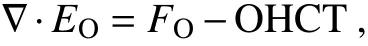
whereFO=FS-Ficeis the energy entering the ocean andFiceis the energy associated with sea ice formation and melting and is calculated from five ensemble members of ECMWF’s ORAS5 (Ocean ReAnalysis System 5) reanalysis(Zuo et al., 2019). OHCT is calculated from OHC (Ocean Heat Content) using central differences (e.g., the OHCT in February is the difference of OHCs between March and January divided by the time difference). The OHCT calculated by Liu et al. (2020) using the OHC integrated over 0-2000 m is used in this study, since it shows good agreement in both absolute value and variability with the global meanFS.The ORAS5 is a state-of-the-art eddy-permitting ocean reanalysis running on (1/4)° resolution. The ORAS5 has been validated, and it is found to provide realistic variability in ocean heat storage and oceanic transports in the tropics (Mayer et al., 2018; Trenberth and Zhang, 2019) and the Arctic(Mayer et al., 2019; Uotila et al., 2019). Considering that the oceanic heat transport is zero at the boudary and the heat transport through the Bering Strait is small and can be neglected (Koenigk and Brodeau, 2014), the oceanic heat transport at different latitudes in the North Atlantic can be accurately estimated by integration from the North Pole.

The AMIP6 and high resolution highresSST-present climate model simulations have prescribed observed sea surface temperature (SST) and sea ice and realistic radiation forcings(Eyring et al., 2016). The highresSST-present is defined in the framework of HighResMIP (Haarsma et al., 2016) and a configuration available in the CMIP6 archive similar to AMIP6, but with a higher horizontal resolution. The highresSST-present experiment is designed to allow for an evaluation of the sensitivity of climate model output to spatial resolution, and to help understand the origins of model biases.The net surface fluxes from these model simulations are calculated by summing up four components of surface latent heat flux, sensible heat flux, and shortwave and longwave radiative fluxes. There are nineteen AMIP6 models and eight highresSST-present models used in this study. Unless stated otherwise, the AMIP6 data include both normal AMIP6 and highresSST-present simulations. The datasets used in this study are listed in Table 1, with brief descriptions.

Table 1. Datasets and brief descriptions.

3.Results

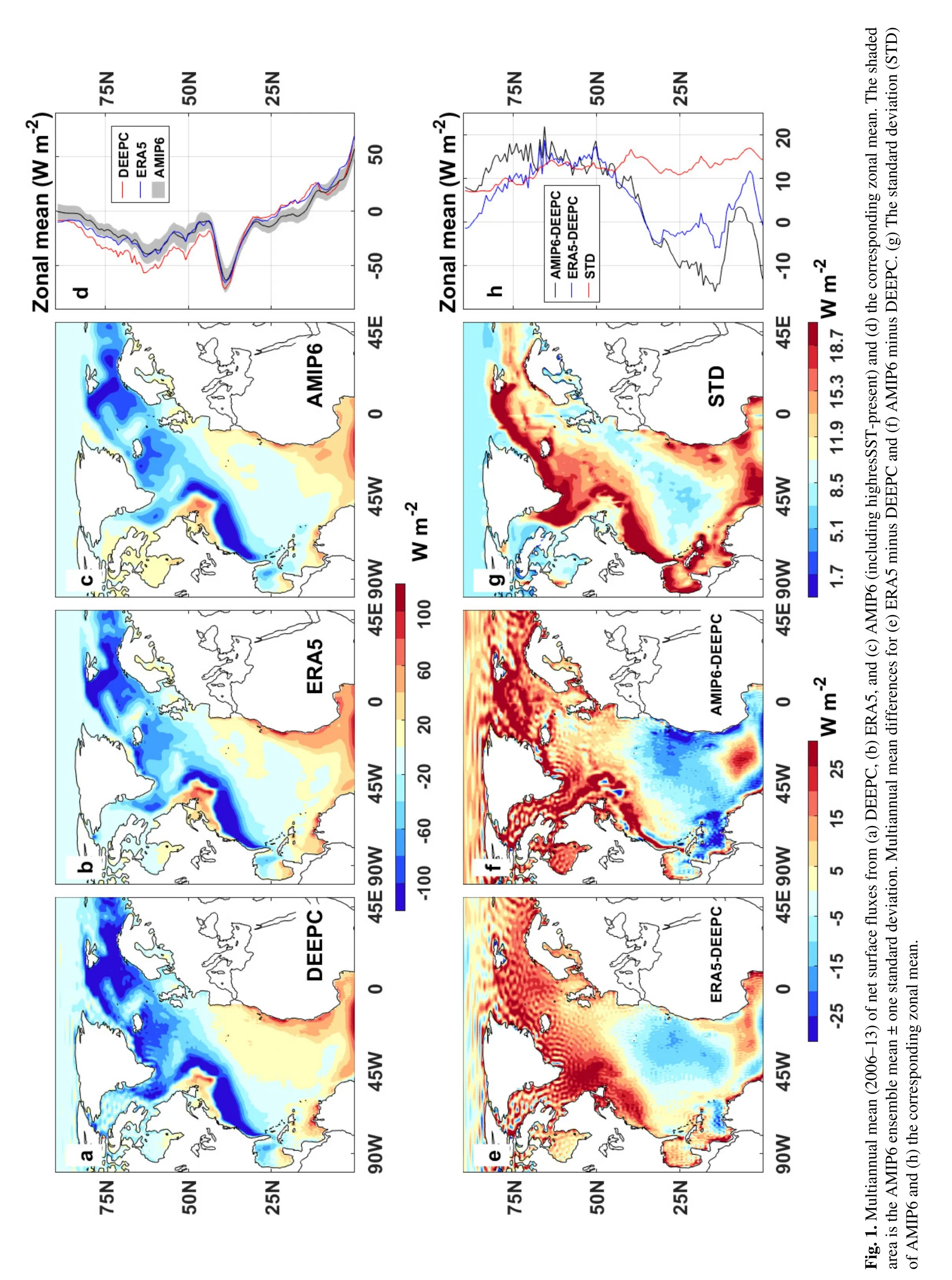
The multiannual mean (2006-13) of ocean net surface heat fluxes in the North Atlantic from DEEPC, ERA5, and AMIP6 (including highresSST-present) are plotted in Figs. 1a-c. It can be seen that, in general, the North Atlantic loses heat to the atmosphere, particularly over the Gulf Stream and the high latitudes. This loss is compensated by the oceanic heat transport from the low latitudes to the high latitudes in the Atlantic. The corresponding zonal means are plotted in Fig. 1d. The shaded area is the AMIP6 ensemble mean ± one standard deviation (STD). The maximum heat loss is at 39°N, where the heat fluxes are 71, 66, and 63 W m-2from DEEPC, ERA5, and the AMIP6 ensemble mean,respectively. The DEEPC data show more heat loss than the AMIP6 ensemble mean north of 35°N, implying more oceanic heat transport is needed to compensate this loss.

The differences in Fig. 1e (ERA5 minus DEEPC) and Fig. 1f (AMIP6 minus DEEPC) show similar large discrepancies over the mid-high latitudes. However, it must be borne in mind that the AMIP6 models have prescribed observed SST and sea ice and realistic radiative forcings; therefore,the atmospheric internal component ofFSis mostly removed when taking the ensemble mean, which is primarily the atmospheric response to the prescribed forcings. Meanwhile, theFSfrom the DEEPC product includes both the atmospheric internal component and the atmospheric response to the prescribed forcings; thus, theFSdifference between DEEPC and the AMIP6 ensemble mean may not indicate the discrepancy ofFSbetween them, but may be largely due to the atmospheric internal component ofFS,which was found to be critical in forcing the oceanic variability in the mid-high-latitude North Atlantic (Barsugli and Battisti, 1998; Delworth and Greatbatch, 2000; Dong and Sutton, 2005; Kwon and Frankignoul, 2012; Colfescu and Schneider, 2020; Chen et al., 2021). However, after checking the difference between DEEPC and individual AMIP6 models, spatial patterns similar to Figs. 1e and 1f are found (not shown).

The large discrepancy region also displays a large STD of the AMIP6 ensemble, as shown in Fig. 1g, with the exception of the area around the Arctic region whereFSis constrained to be close to zero. The STD along the western boundary current, such as in the slope regions of the Greenland Ocean and in the Gulf Stream, is large because of the intense mesoscale activity there (Chelton and Xie, 2010;Putrasahan et al., 2013; Roberts et al., 2017). The ocean eddy activity will affect the turbulent heat fluxes (Roberts et al., 2016), but it cannot be well represented by the prescribed SST over these regions. The zonal mean in Fig. 1h shows that the mean heat loss from DEEPC between 50°-75°N is about 15 W m-2more than that from ERA5 and 13 W m-2more than simulated by the AMIP6 ensemble mean. The dif-ference between DEEPC and the individual AMIP6 model is also examined (not shown), and it is found that 74% of these models (20 out of 27 models) show differences between 9-25 W m-2over 50°-75°N. The mean STD of the AMIP6 net surface heat flux over 50°-75°N is about 12 W m-2. The heat loss averaged over the region north of 26°N from the AMIP6 ensemble mean is about 10 W m-2less than that from DEEPC, and the STD of the difference between DEEPC and AMIP6 models is about 4.3 W m-2.The deseasonalized time series of the area mean ocean net surface heat flux north of 26°N is plotted in Fig. 2. Both DEEPC and the AMIP6 ensemble mean show more-or-less consistent decadal variability after 1995, such as the decrease over 2002-08 and the increase after 2010. The DEEPC estimate does not have a significant trend, but the AMIP6 ensemble mean has a significant trend of -0.34 (W m-2) per decade. The inferior agreement in the interannual variability between DEEPC and the AMIP6 ensemble mean is partly due to the aforementioned atmospheric internal component ofFS. Different horizontal resolutions of AMIP6 models may also play an important role and will be further discussed below. AMIP6 models have prescribed sea ice, but in the real world the sea ice at high latitudes can not only insulate and impede the heat loss from the ocean to the atmosphere, but also can alter the water salinity by the brine rejection during the sea ice formation, therefore increasing the water density and influencing the AMOC and ocean current (Jansen, 2017), affecting the turbulent fluxes. The variability of ERA5 shows less consistency with DEEPC and the AMIP6 ensemble mean, mainly due to the imbalance of the wind-induced mass transport and surface pressure changes, which arises from the lack of observational constraint on divergent winds (Trenberth et al., 2009; Mayer and Haimberger, 2012; Liu et al., 2015, 2020).

Fig. 2. Deseasonalized time series of the area mean ocean net surface heat flux north of 26°N in the Atlantic. The shaded area is the AMIP6 ensemble mean (solid black line) ± one standard deviation. All lines are twelve-month running means.

As an indirect check of the ocean net surface heat fluxes in the North Atlantic, the multiannual mean(2006-13) meridional heat transport is integrated from the North Pole using the above equation from different datasets of net surface heat fluxes, including the DEEPC, ERA5, and nineteen AMIP6 and eight highresSST-present climate model simulations. The sea ice and OHCT are from the ORAS5 ocean reanalysis. The results are shown in Fig. 3.Grey lines are the heat transport from individual AMIP6 simulations, and the ensemble mean is the solid black line. The symbols represent short-term historical observations from various sources and the bars are one standard deviation of multiple measurements (Macdonald, 1998; Bryden and Imawaki,2001; Ganachaud and Wunsch, 2003; Talley, 2003; Lumpkin and Speer, 2007; Johns et al., 2011). The vertical dashed red line shows the location of 26°N. It can be seen that the transport from most of the AMIP6 members is lower than that inferred from DEEPC in the area north of 26°N. Only one member has a heat transport comparable with that inferred from DEEPC, implying that the area meanFSfrom AMIP6 in the area north of 26°N is higher than the estimated DEEPC product (i.e., less heat loss). The inferred AMIP6 ensemble mean oceanic heat transport in the Atlantic is comparable with that inferred from the direct ERA5 surface fluxes in the area north of 26°N, but is much lower than that of DEEPC. The heat transport from AMIP6 spreads quickly after starting the integration from the North Pole, indicating the large spread of the simulatedFSin the North Atlantic,since bothFiceand OHCT are all from the ORAS5. The AMIP6 ensemble mean is closer to DEEPC in the Southern Hemisphere, but it is still about 0.3-0.4 PW lower. The oceanic heat transport inferred from direct ERA5 surface heat flux in the Southern Hemisphere is nearly at the lower end of that from the AMIP6 ensemble.

The time series of the oceanic heat transport at 26°N is plotted in Fig. 4. The inferred heat transport from DEEPC shows reasonable agreement with the RAPID observation in both variability and quantity. The correlation coefficient over the RAPID period (April 2004 to February 2017 in this study) is 0.32, and the mean heat transports are 1.21 PW for RAPID and 1.24 PW for DEEPC, respectively. The earlier trend of RAPID data from 2006-08 is subject to greater uncertainty in observations (Trenberth and Fasullo, 2018; Trenberth et al., 2019). The variability agreement is better after 2008, and the correlation coefficient is 0.73 over 2008-16.The transport inferred directly from the ERA5 surface heat fluxes is much lower than that from DEEPC, even though it is higher than that from ERA-Interim, which is about 0.66 PW over 2004-16 (Liu et al., 2020). There is good agreement in both the variability and quantity of the heat transport between the AMIP6 ensemble mean and ERA5. The correlation coefficient is 0.66, and the mean transports are all 0.91 PW over 1985-2014. The correlation coefficient between DEEPC and AMIP6 is 0.73 over the same period.

Fig. 3. Multiannual mean (2006-13) northward total meridional oceanic heat transports (unit is PW) in the Atlantic derived from net DEEPC surface fluxes, ORAS5 sea ice, and OHCT, together with some short-term historical observations (symbols,error bars show one standard deviation) and those inferred from ERA5 and AMIP6 model surface fluxes (including nineteen AMIP6 and eight highresSST-present model simulations). The vertical dashed red line shows the location of 26°N.

The spread ofFSis large between AMIP6 model simulations because of different subgrid-scale parameterizations in the model dynamics, such as the cumulus convection, cloud microphysics, turbulence, radiation, and land-surface processes. However, the model resolution may play a role. The resolution effects on the multiannual (2006-13) area meanFSover the globe and the ocean area north of 26°N in the Atlantic are plotted in Figs. 5a and 5b, respectively. The effect on the oceanic heat transport at 26°N is plotted in Fig. 5c. Figure 5a shows the decrease of the global area meanFSwith the increase of the model grid-point distance.Model 5 (CanESM) behaves differently. The regression slopes arem= -1.57±1.40 W m-2andm= -0.48±1.21 W m-2per degree horizontal resolution without and with model 5 counted, respectively. The correlation coefficients between theFSand latitudinal resolution arer= -0.43 and-0.16 without and with model 5 counted, respectively. For the region north of 26°N in the Atlantic, the heat loss increases with the increase of the model resolution. The regression slopes arem= 5.47±3.56 andm= 3.63±2.88 W m-2per degree resolution without and with model 5 counted,respectively. The influence of model 5 onFSnorth of 26°N is not as large as that for the global mean. The corresponding correlation coefficients between the meanFSnorth of 26°N and the latitudinal resolution arer= 0.54 and 0.46, respectively. Based on the above equation, it is expected that the relationship betweenFSand model resolution should be the opposite of that between the oceanic heat transport and the resolution. This is shown in Fig. 5c. The heat transport at 26°N increases with the increasing model resolution. The regression slopes arem= -0.22±0.13 andm= -0.15±0.10 PW per degree resolution without and with model 5 counted, and the corresponding correlation coefficients between the heat transport at 26°N and the latitudinal resolution arer= -0.59 and -0.52, respectively. It is observed that when the model resolution is high enough, the heat transport can be comparable with that inferred from DEEPC products.

To investigate the causes of the resolution dependence ofFSin the global mean and north of 26°N in the Atlantic,the dependence of flux components at TOA and surface on the resolution has been plotted in Fig. 6. For global mean TOA radiative fluxes, the RSW (Reflected Shortwave Radiation) decreases with increasing resolution (Fig. 6a), but more OLR (Outgoing Longwave Radiation) leaves the TOA to compensate for it to some extent (Fig. 6b). The net effect is that the radiation flux entering the TOA (FT) increases with higher resolution (Fig. 6c). These results are consistent with Vannière et al. (2019), which used a different set of climate models. Due to the small atmospheric heating capacity and no horizontal divergence for the global mean, most of the energy enetering the TOA will reach the surface. There is a strong correlation betweenFTandFS(Fig. 6d); therefore, the global meanFSalso increases with the higher resolution (Fig. 5a). The physical processes leading to the global area mean RSW and OLR dependence on the model resolution are complicated due to the bias compensation between different regions (Moreno-Chamarro et al., 2022). The increase of OLR and the decrease of RSW with the higher model horizontal resolution are primarily due to a change of cloud radiative forcings in regions of mean ascending motion. Vannière et al. (2019) suggested a possible explanation: at higher resolution, high intensity precipitation events are generated by more compact and more intense convective systems, thus reducing the mean cloud fraction. A more detailed analysis of cloud radiative properties is beyond the scope of this study but will be the object of a future study.

Fig. 4. Northward meridional ocean heat transports at 26°N in the Atlantic from RAPID observations and DEEPC net surface fluxes taking into account sea ice melting and ocean heat storage of ORAS5 0-2000 m, together with the transports inferred from ERA5 surface fluxes (dashed magenta). Grey shading is AMIP6 member mean ± one standard deviation. All lines are twelve-month running means.

ForFSin the region north of 26°N in the Atlantic, four flux components are assessed, and it is found that latent heat(LH) has a similar resolution dependence withFS, as shown in Fig. 6e. Figure 6f shows the scatter plot between the area meanFSand LH (both over the region north of 26°N in the Atlantic). The same range for both axes is selected, so the contribution of LH change toFSchange can be clearly seen.The increase of surface evaporation with increasing resolution has been reported by Vannière et al. (2019) and is a global feature. One possible cause of this is the increase of SW radiation at the surface due to the reduction of the mean cloud fraction(Demory et al., 2014). However, as the sea surface temperature is prescribed in AMIP6 simulations, it cannot relate the increase of incoming shortwave radiation to the surface latent heat flux. Another possible cause is the stronger surface wind speed (Terai et al., 2018), which will affect the relative motion between the wind at 10 m and the ocean surface current and influence the turbulent heat fluxes based on the bulk formula. The sea ice drift at high latitudes can also influence the relative motion in the ocean surface and hence the surface heat flux. Therefore, the ocean surface wind and the sea ice drift may also play roles contributing to the discrepancy of the ocean surface heat flux, as show in previous studies (Wu et al., 2017, 2021b). Additionally, high-frequency atmospheric activity, such as storms, also can contribute to the discrepancy in the simulated ocean net surface heat flux(Condron and Renfrew, 2013; Holdsworth and Myers,2015; Wu et al., 2016, 2020). More dedicated studies would be needed to determine the mechanism causing the increase of LH with increasing resolution across models (Vannière et al., 2019).

Fig. 5. Model resolution effect on multiannual mean (2006-13) net surface flux (a) globally and (b) over the region north of 26°N in the Atlantic. (c) The effect on the oceanic heat transport at 26°N in the Atlantic. Circles with numbers inside represent AMIP6 (red for highresSST) model simulations, and the solid circle is from DEEPC. Correlation coefficients and the regression slopes are also displayed. The thin line and values in the bracket are with model 5 counted.

Fig. 6. Model resolution effect on multiannual (2006-13) global mean (a) RSW, (b) OLR, and (c) FT. (e) The LH over the region north of 26°N in the Atlantic. (d) The scatter plot between global mean FT and FS. (f) The scatter plot between LH and FS over the region north of 26°N in the Atlantic. Model numbers are in the circles. The regression slopes are also displayed. The thin line and values in the bracket are with model 5 counted.

4.Discussion and conclusions

The North Atlantic net surface heat flux plays an important role in the climate system. It can affect the AMOC variation and climate change on the global scale. However, direct observations ofFSover the North Atlantic are sparse; therefore, the estimatedFSfrom DEEPC using the residual method (Liu et al., 2020) has been used as the “truth” in this study. DEEPC products have been widely used in the community for climate research and model validation (Valdivieso et al., 2015; Williams et al., 2015; Roberts et al., 2016,2017; Senior et al., 2016; Hyder et al., 2018; Mignac et al.,2018; Cheng et al., 2019; Trenberth et al., 2019; Allison et al., 2020; Bryden et al., 2020; Mayer et al., 2021, 2022).The latest DEEPC (version 5) product uses the mass-corrected total atmospheric energy divergence from the latest ECMWF release of ERA5 atmospheric reanalysis (Mayer et al., 2021). By combining it with the sea ice data and OHCT from the ECMWF ORAS5 ocean reanalysis, the net heat flux entering the ocean (FO) is estimated and the oceanic heat transport in the Atlantic is calculated.

AMIP6 data, including the highresSST-present datasets,have been widely used for climate research. The ocean net surface heat flux in the North Atlantic from AMIP6 is compared with the DEEPC product in this study to check the discrepancy. There is a large spread of net surface heat fluxes among AMIP6 models. The AMIP6 surface heat loss to the atmosphere is less than that from the DEEPC product (Fig.1). The inferred oceanic heat transport in the Atlantic is calculated and compared with observations as an indirect check of the net surface heat flux. When integrated from the North Pole to 26°N in the Atlantic, heat transports from all AMIP6 models are lower than that from the DEEPC product, and the AMIP6 ensemble mean is close to that inferred from direct ERA5 surface heat fluxes. The integrated heat transport from AMIP6 spreads quickly, implying a large spread in zonal distribution of the net surface heat fluxes, as shown in Fig. 1h. The time series of the heat transport at 26°N across the Atlantic shows good agreement in variability and magnitude between DEEPC and RAPID observations. The mean heat transports are 1.21 PW for RAPID and 1.24 PW for DEEPC, respectively, over the RAPID observation period.The agreement in variability between them is better after 2008, and the correlation coefficient is 0.73 over 2008-16.The inferred heat transports from AMIP6 and ERA5 agree with each other in terms of variability and magnitude, but they are all about 0.3 PW lower than the DEEPC observation-based estimate. It is noticed that the inferred heat transport from direct ERA5 surface heat fluxes is higher than that from ERA-Interim estimated by Liu et al. (2020).

The effect of model resolution on the net surface heat flux and heat transport has been investigated. Results show that the higher resolution did improve the agreement with observations of net surface heat fluxes over the area north of 26°N in the Atlantic, as well as the inferred heat transport.The global meanFSincreases with the increase of the resolution, and the regression slope is about -1.57 W m-2per degree resolution (i.e., the higher the resolution, the higher theFS). Further investigation found that the RSW decreases with increasing resolution (Fig. 6a), primarily due to a change of cloud radiative forcings in regions of mean ascending motion. Vannière et al. (2019) suggested that at higher resolution, high-intensity precipitation events are generated by more compact and more intense convective systems, thus reducing the mean cloud fraction. It merits a more detailed analysis and will be the objective of a future study. Since the atmospheric heat capacity is small, the global mean net TOA radiative fluxFTand net surface heat fluxFSare approximately balanced (Fig. 6d). Therefore, the global meanFSwill also increase with the higher model horizontal resolution.

The correlation coefficient (r= 0.54) between the area meanFSnorth of 26°N in the Atlantic and the model horizontal resolution is significant using a two-tailed test and Pearson critical values at the 5% significance level. The regression slope is about 5.47 W m-2per degree resolution (Fig. 5b),implying more heat loss when the resolution is increased. Further investigation showed that the surface latent heat flux component displays similar resolution dependence to the regional total surface heat flux,FS(Figs. 6e-f). One possible cause is the stronger surface wind speed (Terai et al., 2018),which will affect the relative motion between the wind at 10 m and the ocean surface current and influence the turbulent heat fluxes based on the bulk formula. The sea ice drift at high latitudes can also influence the relative motion in the ocean surface and hence the surface heat flux. Therefore,the ocean surface wind and the sea ice drift may also contribute to the discrepancy of the ocean surface heat flux(Wu et al., 2017, 2021b). Furthermore, high-frequency atmospheric activity, such as storms, also contributes to the discrepancy in the simulated net ocean surface heat flux (Condron and Renfrew, 2013; Holdsworth and Myers, 2015; Wu et al., 2016, 2020). AMIP6 models have prescribed sea ice,but in the real world, sea ice at high latitudes can alter the water salinity by the brine rejection during the sea ice formation, therefore increasing the water density and influencing the AMOC and ocean current (Jansen, 2017), affecting the turbulent fluxes. More dedicated studies focusing on surface ocean processes and cloud radiative forcing should be conducted in the future (Vannière et al., 2019).

As expected, the regression slope between the heat transport at 26°N and the resolution is about -0.22 PW per degree (Fig. 5c), indicating the higher the resolution, the greater the heat transport. The deviation of the AMIP6 heat transport from DEEPC and RAPID is also partly due to the difference in global mean net surface fluxes of AMIP6 simulations. However, the spread of the global area meanFSis about 6.12 W m-2, while theFSspread of 17.59 W m-2over the region north of 26°N in the Atlantic is much larger. Therefore, even when the global mean net surface fluxes from AMIP6 are constrained by the DEEPC product, the reduction in the spread of heat transport will be limited. This remains a challenge for the modeling community. In order to have a deep understanding of the discrepancy between model simulations and observations, further research is needed. These findings can help the research community more accurately interpret the historical simulations and projections produced by contemporary models. By using the ocean current and temperature from the coupled CMIP6 model simulations, the link between the ocean net surface heat fluxes and the oceanic heat transport can be further investigated.

Acknowledgements. This work is supported by the National Natural Science Foundation of China (Grant No. 42075036),Fujian Key Laboratory of Severe Weather (Grant No.2021KFKT02), and the scientific research start-up grant of Guangdong Ocean University (Grant No. R20001). Chunlei LIU is also supported by the University of Reading as a visiting fellow.Richard Allan is supported by the UK National Centre for Earth Observation Grant No. NE/RO16518/1. The DEEPC data are available at https://doi.org/10.17864/1947.000347, the RAPID data can be downloaded from https://rapid.ac.uk/rapidmoc/rapid_data/datadl.php, the ORAS5 data can be accessed from https://www.cen.uni-hamburg.de/icdc/data/ocean/easy-init-ocean/ecmwf-oras5.html, and the AMIP6 data are available from https://esgf-node.llnl.gov/projects/cmip6/. We acknowledge all teams and climate modeling groups for making their data available.